Transcription of Introduction to Queueing Theory
1 Introduction to Queueing Theory Raj Jain Washington University in Saint Louis or A Mini-Course offered at UC Berkeley, Sept-Oct 2012. These slides and audio/video recordings are available on-line at: and ~jain/queue UC Berkeley, Fall 2012 2012 Raj Jain 30-1. Overview Queueing Notation Rules for All Queues Little's Law Types of Stochastic Processes UC Berkeley, Fall 2012 2012 Raj Jain 30-2. Basic Components of a Queue 1. Arrival 6. Service 2. Service time process discipline distribution 5. Population Size 4. Waiting positions 3. Number of servers UC Berkeley, Fall 2012 2012 Raj Jain 30-3. Kendall Notation A/S/m/B/K/SD.
2 A: Arrival process S: Service time distribution m: Number of servers B: Number of buffers (system capacity). K: Population size, and SD: Service discipline UC Berkeley, Fall 2012 2012 Raj Jain 30-4. Arrival Process Arrival times: Interarrival times: j form a sequence of Independent and Identically Distributed (IID) random variables Notation: M = Memoryless Exponential E = Erlang H = Hyper-exponential D = Deterministic constant G = General Results valid for all distributions UC Berkeley, Fall 2012 2012 Raj Jain 30-5. Service Time Distribution Time each student spends at the terminal. Service times are IID.
3 Distribution: M, E, H, D, or G. Device = Service center = Queue Buffer = Waiting positions UC Berkeley, Fall 2012 2012 Raj Jain 30-6. Service Disciplines First-Come-First-Served (FCFS). Last-Come-First-Served (LCFS) = Stack (used in 9-1-1 calls). Last-Come-First-Served with Preempt and Resume (LCFS-PR). Round-Robin (RR) with a fixed quantum. Small Quantum Processor Sharing (PS). Infinite Server: (IS) = fixed delay Shortest Processing Time first (SPT). Shortest Remaining Processing Time first (SRPT). Shortest Expected Processing Time first (SEPT). Shortest Expected Remaining Processing Time first (SERPT).
4 Biggest-In-First-Served (BIFS). Loudest-Voice-First-Served (LVFS). UC Berkeley, Fall 2012 2012 Raj Jain 30-7. Example M/M/3/20/1500/FCFS. Time between successive arrivals is exponentially distributed. Service times are exponentially distributed. Three servers 20 Buffers = 3 service + 17 waiting After 20, all arriving jobs are lost Total of 1500 jobs that can be serviced. Service discipline is first-come-first-served. Defaults: Infinite buffer capacity Infinite population size FCFS service discipline. G/G/1 = G/G/1/ / /FCFS. UC Berkeley, Fall 2012 2012 Raj Jain 30-8. Quiz 30A. Key: A/S/m/B/K/SD.
5 TF. The number of servers in a M/M/1/3 queue is 3. G/G/1/30/300/LCFS queue is like a stack M/D/3/30 queue has 30 buffers G/G/1 queue has population size D/D/1 queue has FCFS discipline UC Berkeley, Fall 2012 2012 Raj Jain 30-9. Exponential Distribution Probability Density Function (pdf): 1. a 1 x/a f(x). f (x) = e a Cumulative Distribution x Z xFunction (cdf): 1. F (x) = P (X < x) = f (x)dx = 1 e x/a 0 F(x). Mean: a x Variance: a2. Coefficient of Variation = (Std Deviation)/mean = 1. Memoryless: Expected time to the next arrival is always a regardless of the time since the last arrival Remembering the past history does not help.
6 UC Berkeley, Fall 2012 2012 Raj Jain 30-11. Erlang Distribution Sum of k exponential random variables 1 k Series of k servers with exponential service times Xk X= xi where xi exponential i=1. Probability Density Function (pdf): xk 1 e x/a f (x) =. (k 1)!ak Expected Value: ak Variance: a2k CoV: 1/ k UC Berkeley, Fall 2012 2012 Raj Jain 30-12. Hyper-Exponential Distribution The variable takes ith value with probability pi x1. x x2.. xm xi is exponentially distributed with mean ai Higher variance than exponential Coefficient of variation > 1. UC Berkeley, Fall 2012 2012 Raj Jain 30-13. Group Arrivals/Service Bulk arrivals/service M[x]: x represents the group size G[x]: a bulk arrival or service process with general inter-group times.
7 Examples: M[x]/M/1 : Single server queue with bulk Poisson arrivals and exponential service times M/G[x]/m: Poisson arrival process, bulk service with general service time distribution, and m servers. UC Berkeley, Fall 2012 2012 Raj Jain 30-14. Quiz 30B. Exponential distribution is denoted as ___. _____ distribution represents a set of parallel exponential servers Erlang distribution Ek with k=1 is same as _____. distribution UC Berkeley, Fall 2012 2012 Raj Jain 30-15. Key Variables 1. 2.. m nq ns n Previous Begin End Arrival Arrival Service Service Time w s r UC Berkeley, Fall 2012 2012 Raj Jain 30-17.
8 Key Variables (cont). Inter-arrival time = time between two successive arrivals. Mean arrival rate = 1/E[ ]. May be a function of the state of the system, , number of jobs already in the system. s = Service time per job. = Mean service rate per server = 1/E[s]. Total service rate for m servers is m . n = Number of jobs in the system. This is also called queue length. Note: Queue length includes jobs currently receiving service as well as those waiting in the queue. UC Berkeley, Fall 2012 2012 Raj Jain 30-18. Key Variables (cont). nq = Number of jobs waiting ns = Number of jobs receiving service r = Response time or the time in the system = time waiting + time receiving service w = Waiting time = Time between arrival and beginning of service UC Berkeley, Fall 2012 2012 Raj Jain 30-19.
9 Rules for All Queues Rules: The following apply to G/G/m queues 1. Stability Condition: Arrival rate must be less than service rate < m . Finite-population or finite-buffer systems are always stable. Instability = infinite queue Sufficient but not necessary. D/D/1 queue is stable at = . 2. Number in System versus Number in Queue: n = nq+ ns Notice that n, nq, and ns are random variables. E[n]=E[nq]+E[ns]. If the service rate is independent of the number in the queue, Cov(nq,ns) = 0. UC Berkeley, Fall 2012 2012 Raj Jain 30-20. Rules for All Queues (cont). 3. Number versus Time: If jobs are not lost due to insufficient buffers, Mean number of jobs in the system = Arrival rate Mean response time 4.
10 Similarly, Mean number of jobs in the queue = Arrival rate Mean waiting time This is known as Little's law. 5. Time in System versus Time in Queue r=w+s r, w, and s are random variables. E[r] = E[w] + E[s]. UC Berkeley, Fall 2012 2012 Raj Jain 30-21. Rules for All Queues(cont). 6. If the service rate is independent of the number of jobs in the queue, Cov(w,s)=0. UC Berkeley, Fall 2012 2012 Raj Jain 30-22. Quiz 30C. If a queue has 2 persons waiting for service, the number is system is ____. If the arrival rate is 2 jobs/second, the mean inter- arrival time is _____ second. In a 3 server queue, the jobs arrive at the rate of 1.