Transcription of Introduction to Time Series Analysis. Lecture 1.
1 Introduction to Time Series Analysis. Lecture Bartlett1. Organizational Objectives of time Series analysis. Overview of the Time Series Time Series modelling: Chasing Issues Peter Bartlett. Office hours: Tue 11-12, Thu10-11(Evans 399). Joe Neeman. Office hours: Wed 1:30 2:30, Fri 2-3(Evans ???). bartlett/courses/153-fall2010/Check it for announcements, assignments, slides, .. Text:Time Series Analysis and its Applications. With R Examples,Shumway and Stoffer. 2nd Edition. IssuesClassroom and Computer Lab Section:Friday 9 11, in 344 tomorrow, August 27:Sign up for computer accounts. Introduction to :Lab/Homework Assignments (25%): posted on the involve a mix of pen-and-paper and computer exercises. You may useany programming language you choose (R, Splus, Matlab, python).Midterm Exams (30%): scheduled for October 7 and November 9,at (10%): Analysis of a data set that you Exam (35%): scheduled for Friday, December Time Series0100020003000400050006000700005010 01502002503003504004A Time Series1960196519701975198019851990050100 150200250300350400year5A Time Series1960196519701975198019851990050100 150200250300350400year$6A Time Series1960196519701975198019851990050100 150200250300350400year$SP500: 1960 19907A Time $SP500: Jan Jun 19878A Time Series2402502602702802903003100510152025 30$SP500 Jan Jun 1987.
2 Histogram9A Time Series0204060801001202202402602803003203 40$SP500: Jan Jun 1987. of Time Series Analysis1. Compact description of Hypothesis decomposition: An exampleMonthly sales for a souvenir shop at a beach resort town in Queensland.(Makridakis, Wheelwright and Hyndman, 1998)0102030405060708090024681012x 10412 Transformed 1 and seasonal of Time Series Analysis1. Compact description of : Classical decomposition:Xt=Tt+St+ : Seasonal : Predict Hypothesis dataMonthly number of unemployed people in Australia.(Hipel and McLeod, 1994) 10519 Trend plus seasonal 10520 Residuals1983198419851986198719881989199 0 6 4 202468x 10421 Predictions based on a (simulated) 10522 Objectives of Time Series Analysis1. Compact description of data:Xt=Tt+St+f(Yt) + : Seasonal : Predict : Impact of monetary policy on Hypothesis : Global : Estimate probability of catastrophic of the Course1.
3 Time Series models2. Time domain methods3. Spectral analysis4. State space models(?)24 Overview of the Course1. Time Series models(a) Stationarity.(b) Autocorrelation function.(c) Transforming to Time domain methods3. Spectral analysis4. State space models(?)25 Overview of the Course1. Time Series models2. Time domain methods(a) AR/MA/ARMA models.(b) ACF and partial autocorrelation function.(c) Forecasting(d) Parameter estimation (e) ARIMA models/seasonal ARIMA models3. Spectral analysis4. State space models(?)26 Overview of the Course1. Time Series models2. Time domain methods3. Spectral analysis(a) Spectral density(b) Periodogram(c) Spectral estimation4. State space models(?)27 Overview of the Course1. Time Series models2. Time domain methods3. Spectral analysis4. State space models(?)(a) ARMAX models.(b) Forecasting, Kalman filter.(c) Parameter Series ModelsAtime Series modelspecifies the joint distribution of the se-quence{Xt}of random example:P[X1 x1.]
4 , Xt xt]for alltandx1, .. , :X1, X2, ..is a stochastic , x2, ..is a single ll mostly restrict our attention tosecond-order propertiesonly:EXt,E(Xt1, Xt2).29 Time Series ModelsExample: White noise:Xt W N(0, 2). ,{Xt}uncorrelated, EXt= 0, VarXt= : noise:{Xt}independent and identically [X1 x1, .. , Xt xt] =P[X1 x1] P[Xt xt].Not interesting for forecasting:P[Xt xt|X1, .. , Xt 1] =P[Xt xt].30 Gaussian white noiseP[Xt xt] = (xt) =1 2 xt e x2 2 1 white noise05101520253035404550 2 1 Series ModelsExample: Binary [Xt= 1] =P[Xt= 1] = 1 1 walkSt= ti= : St=St St 1= 4 20246834 Random walkESt? VarSt?05101520253035404550 15 10 5051035 Random WalkRecall S&P500 data.(Notice that it s smooth) $SP500: Jan Jun 198736 Random WalkDifferences: St=St St 1= 10 8 6 4 20246810year$SP500, Jan Jun 1987. first differences37 Trend and Seasonal ModelsXt=Tt+St+Et= 0+ 1t+ i( icos( it) + isin( it)) + and Seasonal ModelsXt=Tt+Et= 0+ 1t+ and Seasonal ModelsXt=Tt+St+Et= 0+ 1t+ i( icos( it) + isin( it)) + and Seasonal Models: Residuals050100150200250 Series Modelling1.
5 Plot the time for trends, seasonal components, step changes, Transform data so that residuals arestationary.(a) Estimate and subtractTt, St.(b) Differencing.(c) Nonlinear transformations (log, ).3. Fit model to transformationsRecall: Monthly sales.(Makridakis, Wheelwright and Hyndman, 1998)0102030405060708090024681012x Series Modelling1. Plot the time for trends, seasonal components, step changes, Transform data so that residuals arestationary.(a) Estimate and subtractTt, St.(b) Differencing.(c) Nonlinear transformations (log, ).3. Fit model to : S&P 500 $SP500: Jan Jun 10 8 6 4 20246810year$SP500, Jan Jun 1987. first differences45 Differencing and TrendDefine the lag-1difference operator,(think first derivative ) Xt=Xt Xt 1= (1 B)Xt,whereBis thebackshiftoperator,BXt=Xt 1. IfXt= 0+ 1t+Yt, then Xt= 1+ Yt. IfXt= ki=0 iti+Yt, then kXt=k! k+ kYt,where kXt= ( k 1Xt)and 1Xt= and Seasonal VariationDefine the lag-sdifference operator, sXt=Xt Xt s= (1 Bs)Xt,whereBsis the backshift operator appliedstimes,BsXt=B(Bs 1Xt)andB1Xt= +St+Yt, andSthas periods(that is,St=St sfor allt), then sXt=Tt Tt s+ Series Modelling1.
6 Plot the time for trends, seasonal components, step changes, Transform data so that residuals arestationary.(a) Estimate and subtractTt, St.(b) Differencing.(c) Nonlinear transformations (log, ).3. Fit model to Objectives of time Series analysis. Overview of the Time Series Time Series modelling: Chasing