Transcription of Joint Distribution - Example
1 Lecture 17: Joint DistributionsStatistics 104 Colin RundelMarch 26, 2012 Section Distributions of Discrete RVsJoint Distribution - ExampleDraw two socks at random, without replacement, from a drawer full oftwelve colored socks:6 black, 4 white, 2 purpleLetBbe the number of Black socks,Wthe number of White socksdrawn, then the distributions ofBandWare given by:012P(B=k)612511=15662612611=366661251 1=1566P(W=k)812711=28662412811=326641231 1=666 Note -B HyperGeo(12,6,2) =(6k)(62 k)(122)andW HyperGeo(12,4,2) =(4k)(82 k)(122)Statistics 104 (Colin Rundel)Lecture 17 March 26, 20121 / 32 Section Distributions of Discrete RVsJoint Distribution - Example , the number of Black socks andWthe number of White socksdrawn, then the Joint Distribution ofBandWis given by:W01201668666661566B112662466036662156 6001566286632666666666P(B=b,W=w) = 1/66 If b=0,w=08/66 If b=0,w=16/66 If b=0,w=212/66 If b=1,w=024/66 If b=1,w=10/66 If b=1,w=215/66 If b=2,w=00/66 If b=2,w=10/66 If b=2,w=2P(B=b,W=w) =(6b)(4w)(22 b w)(122), for 0 b,w 2 andb+w 2 Statistics 104 (Colin Rundel)Lecture 17 March 26, 20122 / 32 Section Distributions of Discrete RVsMarginal DistributionsNote that the column and row sums are the distributions (B=b) =P(B=b,W= 0) +P(B=b,W= 1) +P(B=b,W= 2)P(W=w) =P(B= 0,W=w) +P(B= 1,W=w) +P(B= 2,W=w)These are themarginaldistributions ofBandW.
2 In general,P(X=x) = yP(X=x,Y=y) = yP(X=x|Y=y)P(Y=y)Statistics 104 (Colin Rundel)Lecture 17 March 26, 20123 / 32 Section Distributions of Discrete RVsConditional DistributionConditional distributions are defined as we have seen previously withP(X=x|Y=y) =P(X=x,Y=y)P(Y=y)= Joint pmfmarginal pmfTherefore the pmf for white socks given no black socks were drawn isP(W=w|B= 0) =P(W=w,B= 0)P(B= 0)= 166/1566=115ifW= 0866/1566=815ifW= 1666/1566=615ifW= 2 Statistics 104 (Colin Rundel)Lecture 17 March 26, 20124 / 32 Section Distributions of Continuous RVsJoint CDFF(x,y) =P[X x,Y y]=P[(X,Y) lies south-west of the point (x,y)]XYl(x,y)Statistics 104 (Colin Rundel)Lecture 17 March 26, 20125 / 32 Section Distributions of Continuous RVsJoint CDF, Joint Cumulative Distribution function follows the same rules as theunivariate CDF,Univariate definition:F(x) =P(X x) = x f(z)dzlimx F(x) = 0limx F(x) = 1x y F(x) F(y)Bivariate definition:F(x,y) =P(X x,Y y) = y x f(x,y)dx dylimx,y F(x,y) = 0limx,y F(x,y) = 1x x ,y y F(x,y) F(x ,y )Statistics 104 (Colin Rundel)Lecture 17 March 26, 20126 / 32 Section Distributions of Continuous RVsMarginal DistributionsWe can define marginal distributions based on the CDF by setting one ofthe values to infinity:F(x, ) =P(X x,Y ) = x f(x,y)dy dy=P(X x) =FX(x)F( ,y) =P(X ,Y y) = y f(x,y)dx dy=P(Y y) =FY(y)Statistics 104 (Colin Rundel)Lecture 17 March 26, 20127 / 32 Section Distributions of Continuous RVsJoint pdfSimilar to the CDF the probability density function follows the samegeneral rules except in two dimensions,Univariate definition:f(x) 0 for allxf(x) =ddxF(x) f(x)dx= 1 Bivariate definition.
3 F(x,y) 0 for all (x,y)f(x,y) = x yF(x,y) f(x,y)dx dy= 1 Statistics 104 (Colin Rundel)Lecture 17 March 26, 20128 / 32 Section Distributions of Continuous RVsMarginal pdfsMarginal probability density functions are defined in terms of integratingout one of the random (x) = f(x,y)dyfY(x) = f(x,y)dxPreviously we defined independence in terms ofE(XY) =E(X)E(Y) XandYare independent. This is equivalent in the Joint case off(x,y) =fX(x)fY(y) XandYare 104 (Colin Rundel)Lecture 17 March 26, 20129 / 32 Section Distributions of Continuous RVsProbability and ExpectationUnivariate definition:P(X A) = Af(x)dxE[g(X)] = g(x) f(x)dxBivariate definition:P(X A,Y B) = A Bf(x,y)dx dyE[g(X,Y)] = g(x,y) f(x,y)dx dyStatistics 104 (Colin Rundel)Lecture 17 March 26, 201210 / 32 Section Distributions of Continuous RVsExample 1 - Joint UniformsLetX,Y Unif(0,1), it is straight forward to see graphically thatF(x,y) = 0ifx ( ,0) ory ( ,0)xyifx (0,1),y (0,1)xifx (0,1),y (1, )yifx (1, ),y (0,1)1ifx (1, ),y (1, )Statistics 104 (Colin Rundel)Lecture 17 March 26, 201211 / 32 Section Distributions of Continuous RVsExample 1, on the CDF we can calculate the pdf using the 2nd partialderivative with regard to x and (x,y) = x yF(x,y)= 0 ifx ( ,0) ory ( ,0)1 ifx (0,1),y (0,1)0 ifx (0,1),y (1, )0 ifx (1, ),y (0,1)0 ifx (1, ),y (1, )={1 ifx (0,1),y (0,1)0 otherwiseStatistics 104 (Colin Rundel)}
4 Lecture 17 March 26, 201212 / 32 Section Distributions of Continuous RVsExample 1, on the pdf we can calculate the marginal densities:f(x,y) ={1 ifx (0,1),y (0,1)0 otherwisefX(x) = f(x,y)dy={ 101dyifx (0,1) 0dyotherwise={1 ifx (0,1)0 otherwisefY(y) ={1 ify (0,1)0 otherwiseWhich should not be 104 (Colin Rundel)Lecture 17 March 26, 201213 / 32 Section Distributions of Continuous RVsExample 1, is also straight forward:E(X) = xf(x,y)dx dy= 10 10x dx dy= 10(x22 10)dy= 1012dy=12y 10= 1/2E(Y) = yf(x,y)dx dy= 10 10y dx dy= 10(xy|10)dy= 10y dy=y22 10= 1/2 Statistics 104 (Colin Rundel)Lecture 17 March 26, 201214 / 32 Section Distributions of Continuous RVsExample 1, (XY) = xyf(x,y)dx dy= 10 10xy dx dy= 10(x2y2 1x=0)dy= 10y2dy=y24 10= 1/4 Note thatE(XY) =E(X)E(Y), what does this tell us aboutXandY?}}}}
5 Statistics 104 (Colin Rundel)Lecture 17 March 26, 201215 / 32 Section Distributions of Continuous RVsExample 1, another wayIf we did not feel comfortable coming up with the graphical arguments forF(x,y) we can also use the fact that the pdf is constant on (0,1) (0,1)to derive the same Distribution / (x,y) =c1 = f(x,y)dx dy= 10 10c dx dy= 10(cx|10)dy= 10c dy=cy|10=cStatistics 104 (Colin Rundel)Lecture 17 March 26, 201216 / 32 Section Distributions of Continuous RVsExample 2 Let X and Y be drawn uniformly from the triangle belowXY0011223344 Find the Joint pdf, cdf, and 104 (Colin Rundel)Lecture 17 March 26, 201217 / 32 Section Distributions of Continuous RVsExample 2, the Joint density is constant thenf(x,y) =c=29,for 0 x+y 3based on the area of the triangle, but we need to be careful to define onwhat range. We can define the range in two ways sinceXandYdependon each other, so we can define the range ofXin terms ofYorYinterms (x,y) ={29ify (0,3),x (0,3 y)0otherwise={29ifx (0,3),y (0,3 x)0otherwiseStatistics 104 (Colin Rundel)Lecture 17 March 26, 201218 / 32 Section Distributions of Continuous RVsExample 2, on which range definition you choose it makes life easier whenevaluating the marginal (x) = f(x,y)dy= 3 x029dy=29(3 x) forx (0,3)fY(y) = f(x,y)dy= 3 y029dx=29(3 y) fory (0,3)AreXandYindependent?}}
6 Statistics 104 (Colin Rundel)Lecture 17 March 26, 201219 / 32 Section Distributions of Continuous RVsExample 2, the CDF with calculus is hard in this case, still a pain withgraphical approaches but (x,y) = y x f(x,y)dx dy= 0ifx ( ,0) ory ( ,0)29xyifx (0,3),y (0,3),x+y (0,3)29(xy (y (3 x))(x (3 y))2)ifx (0,3),y (0,3),x+y (3,6)29(3x x22)ifx (0,3),y (3, )29(3y y22)ifx (3, ),y (0,3)1ifx (3, ),y (3, )Statistics 104 (Colin Rundel)Lecture 17 March 26, 201220 / 32 Section Distributions of Continuous RVsExample 3 Letf(x,y) =cx2yforx2 y :a)cb)P[X Y]c)fX(x) andfY(y)Statistics 104 (Colin Rundel)Lecture 17 March 26, 201221 / 32 Section Distributions of Continuous RVsExample 3 - RangeXY1 101 Statistics 104 (Colin Rundel)Lecture 17 March 26, 201222 / 32 Section Distributions of Continuous RVsExample (x,y) =cx2yforx2 y 1, we can rewrite the bounds as0 y 1, y x y1 = f(x,y)dx dy= 10 y 1cx2y dx dy= 10(cyx33 yx= y)dy= 10(cy5/2/3 +cy5/2/3)dy=4cy7/221 1y=0=421cc= 21/4 Statistics 104 (Colin Rundel)Lecture 17 March 26, 201223 / 32 Section Distributions of Continuous RVsExample 3 - pdf (x,y) 104 (Colin Rundel)Lecture 17 March 26, 201224 / 32 Section Distributions of Continuous RVsExample need to integrate over the region wherex2 y 1 andx ywhichis indicated in red belowXY1 101XY1 101 Statistics 104 (Colin Rundel)
7 Lecture 17 March 26, 201225 / 32 Section Distributions of Continuous RVsExample , (X Y) = 1 1 |x|x2214x2y dy dx= 2 10 xx2214x2y dy dx=424 10(x2y22 xx2)dx=424 10(x42 x62)dx=424(x510 x714) 10=424(110 114)=424(270)= 104 (Colin Rundel)Lecture 17 March 26, 201226 / 32 Section Distributions of Continuous RVsExample (x) = 1x2214x2y dy=214(x2y22 1x2)=218(x2 x6),forx ( 1,1)fY(y) = y y214x2y dx=214(x3y3 y y)=214(2y5/23)=72y5/2,fory (0,1)Statistics 104 (Colin Rundel)Lecture 17 March 26, 201227 / 32 Section Distributions of Continuous RVsExample , is always a good idea to check that the marginals are proper densities. 1 1fX(x)dx= 1 1218(x2 x6)dx=218(x33 x77) 1 1=214(13 17)= 1 10fY(y)dy= 1072y5/2dy=7227y7/2 10= 1 Statistics 104 (Colin Rundel)Lecture 17 March 26, 201228 / 32 Section Distributions of Continuous RVsExample 4 LetYbe the rate of calls at a help desk, andXthe number of callsbetween 2 pm and 4 pm one day; Let s say that:f(x,y) =(2y)xx!
8 E 3yfory>0,x= 0,1,2,..Find:a)P(X= 0)b)P(Y>2)c)P[X=x] for allxStatistics 104 (Colin Rundel)Lecture 17 March 26, 201229 / 32 Section Distributions of Continuous RVsExample (x,y) =(2y)xx!e 3y,fory>0,x= 0,1,2,..P(X= 0) = 0f(0,y)dy= 0e 3ydy= 13e 3y 0= 1/3 Statistics 104 (Colin Rundel)Lecture 17 March 26, 201230 / 32 Section Distributions of Continuous RVsExample (x,y) =(2y)xx!e 3y,fory>0,x= 0,1,2,..P(Y>2) = 2 x=0f(x,y)dy= 2 x=0(2y)xx!e 3ydy= 2e 3y( x=0(2y)xx!)dy= 2e 3y( x=01 +(2y)1+(2y)22+ )dy= 2e 3y(e2y)dy= 2e ydy= e y 2=e 2= 104 (Colin Rundel)Lecture 17 March 26, 201231 / 32 Section Distributions of Continuous RVsExample (x,y) =(2y)xx!e 3y,fory>0,x= 0,1,2,..P(X=x) = 0f(x,y)dy= 0(2y)xx!e 3ydy=2x3x+1 Statistics 104 (Colin Rundel)Lecture 17 March 26, 201232 / 32