Chapter 5: JOINT PROBABILITY DISTRIBUTIONS Part 1 ...

1 Chapter 5: JOINT PROBABILITY . DISTRIBUTIONS . Part 1: Sections to For both discrete and continuous random variables we will discuss the JOINT DISTRIBUTIONS (for two or more 's). Marginal DISTRIBUTIONS (computed from a JOINT distribution ). Conditional DISTRIBUTIONS ( P (Y = y|X = x)). Independence for 's X and Y. This is a good time to refresh your memory on double-integration. We will be using this skill in the upcom- ing lectures. 1. Recall a discrete PROBABILITY distribution (or pmf ) for a single X with the example be- x 0 1 2. f (x) Sometimes we're simultaneously interested in two or more variables in a random experiment.

2 We're looking for a relationship between the two variables. Examples for discrete 's Year in college vs. Number of credits taken Number of cigarettes smoked per day vs. Day of the week Examples for continuous 's Time when bus driver picks you up vs. Quantity of caffeine in bus driver's system Dosage of a drug (ml) vs. Blood compound measure (percentage). 2. In general, if X and Y are two random variables, the PROBABILITY distribution that defines their si- multaneous behavior is called a JOINT PROBABILITY distribution . Shown here as a table for two discrete random variables, which gives P (X = x, Y = y).

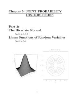
3 X 1 2 3. 1 0 1/6 1/6. y 2 1/6 0 1/6. 3 1/6 1/6 0. Shown here as a graphic for two continuous ran- dom variables as fX,Y (x, y). 3. If X and Y are discrete, this distribution can be described with a JOINT PROBABILITY mass function. If X and Y are continuous, this distribution can be described with a JOINT PROBABILITY density function. Example: Plastic covers for CDs (Discrete JOINT pmf). Measurements for the length and width of a rectangular plastic covers for CDs are rounded to the nearest mm (so they are discrete). Let X denote the length and Y denote the width. The possible values of X are 129, 130, and 131 mm.

4 The possible values of Y are 15 and 16 mm (Thus, both X and Y are discrete). 4. There are 6 possible pairs (X, Y ). We show the PROBABILITY for each pair in the following table: x=length 129 130 131. y=width 15 16 The sum of all the probabilities is The combination with the highest probabil- ity is (130, 15). The combination with the lowest PROBABILITY is (131, 16). The JOINT PROBABILITY mass function is the func- tion fXY (x, y) = P (X = x, Y = y). For example, we have fXY (129, 15) = 5. If we are given a JOINT PROBABILITY distribution for X and Y , we can obtain the individual prob- ability distribution for X or for Y (and these are called the Marginal PROBABILITY Dis- tributions).

5 Example: Continuing plastic covers for CDs Find the PROBABILITY that a CD cover has length of 129mm ( X = 129). x= length 129 130 131. y=width 15 16 P (X = 129) = P (X = 129 and Y = 15). + P (X = 129 and Y = 16). = + = What is the PROBABILITY distribution of X? 6. x= length 129 130 131. y=width 15 16 column totals The PROBABILITY distribution for X appears in the column x 129 130 131. fX (x) . NOTE: We've used a subscript X in the PROBABILITY mass function of X, or fX (x), for clarification since we're considering more than one variable at a time now. 7. We can do the same for the Y random variable: row x= length totals 129 130 131.

6 Y=width 15 16 column totals 1. y 15 16. fY (y) Because the the PROBABILITY mass functions for X and Y appear in the margins of the table ( column and row totals), they are often re- ferred to as the Marginal DISTRIBUTIONS for X and Y . When there are two random variables of inter- est, we also use the term bivariate probabil- ity distribution or bivariate distribution to refer to the JOINT distribution . 8. JOINT PROBABILITY Mass Function The JOINT PROBABILITY mass function of the dis- crete random variables X and Y , denoted as fXY (x, y), satisfies (1) fXY (x, y) 0. XX. (2) fXY (x, y) = 1.

7 X y (3) fXY (x, y) = P (X = x, Y = y). For when the 's are discrete. (Often shown with a 2-way table.). x= length 129 130 131. y=width 15 16 9. Marginal PROBABILITY Mass Function If X and Y are discrete random variables with JOINT PROBABILITY mass function fXY (x, y), then the marginal PROBABILITY mass functions of X and Y are X. fX (x) = fXY (x, y). y and X. fY (y) = fXY (x, y). x where the sum for fX (x) is over all points in the range of (X, Y ) for which X = x and the sum for fY (y) is over all points in the range of (X, Y ) for which Y = y. We found the marginal distribution for X in the CD example x 129 130 131.

8 FX (x) 10. HINT: When asked for E(X) or V (X) ( val- ues related to only 1 of the 2 variables) but you are given a JOINT PROBABILITY distribution , first calculate the marginal distribution fX (x) and work it as we did before for the univariate case ( for a single random variable). Example: Batteries Suppose that 2 batteries are randomly cho- sen without replacement from the following group of 12 batteries: 3 new 4 used (working). 5 defective Let X denote the number of new batteries chosen. Let Y denote the number of used batteries chosen. 11. a) Find fXY (x, y). { the JOINT PROBABILITY distribution }.

9 B) Find E(X). ANS: a) Though X can take on values 0, 1, and 2, and Y can take on values 0, 1, and 2, when we consider them jointly, X + Y 2. So, not all combinations of (X, Y ) are possible. There are 6 possible CASE: no new, no used (so ! all defective). 5. 2. fXY (0, 0) = ! = 10/66. 12. 2. 12. CASE: no new, 1 used ! ! 4 5. 1 1. fXY (0, 1) = ! = 20/66. 12. 2. CASE: no new, 2 used ! 4. 2. fXY (0, 2) = ! = 6/66. 12. 2. CASE: 1 new, no used ! ! 3 5. 1 1. fXY (1, 0) = ! = 15/66. 12. 2. 13. CASE: 2 new, no used ! 3. 2. fXY (2, 0) = ! = 3/66. 12. 2. CASE: 1 new, 1 used ! ! 3 4. 1 1. fXY (1, 1) = !

10 = 12/66. 12. 2. The JOINT distribution for X and Y x= number of new chosen 0 1 2. y=number of 0 10/66 15/66 3/66. used 1 20/66 12/66. chosen 2 6/66. ThereP. are P. 6 possible (X, Y ) pairs. And, x y fXY (x, y) = 1. 14. b) Find E(X). 15. JOINT PROBABILITY Density Function A JOINT PROBABILITY density function for the continuous random variable X and Y , de- noted as fXY (x, y), satisfies the following properties: 1. fXY (x, y) 0 for all x, y R R . 2. fXY (x, y) dx dy = 1. 3. For any region R of 2-D space Z Z. P ((X, Y ) R) = fXY (x, y) dx dy R. For when the 's are continuous. 16. Example: Movement of a particle An article describes a model for the move- ment of a particle.