Transcription of Lecture 4: Diffusion: Fick’s second law
1 1 Lecture 4: diffusion : fick s second law Today s topics Learn how to deduce the fick s second law, and understand the basic meaning, in comparison to the first law. Learn how to apply the second law in several practical cases, including homogenization, interdiffusion in carburization of steel, where diffusion plays dominant role. In last Lecture , we learned fick s first Law: J = -D dxxdc)( (Unit: D: cm2/sec; J: number/cm2/sec) Where D = /RTG-2Ae6 a=61 a2 fick s first law applies to steady state systems, where concentration keeps constant.
2 But in many cases of diffusion , the concentration however changes with time, how to describe the diffusion kinetics in these cases --- demanding fick s second Law. Continued from last Lecture , we will learn how to deduce the fick s second law, and understand the meanings when applied to some practical cases. Let s consider a case like this We can define the local concentration and diffusion flux (through a unit area, A ) at position x as: c (x,t), J(x) we have dc(x) = [()()]dJxJxdxtAAdx +, J(x+dx) = J(x) + dJ x C dx A A j(x) x x+dx j(x+dx) dx 2 then, we have (,)dcxtdt = - dJdx or, rewrite it in this format with replacing d (,)cxtt = - Jx from the first law: J = -D dxxdc)(= -D ()cxx then, we have ttxc ),( = - Jx = D 22xc (1) This is the fick s second law.
3 In three-dimensional space, it can be written as: tc = D c2 . At steady (equilibrium) state, we have (,)cxt /dt = 0 (meaning no concentration change) Then, solving Eq. (1) gives -D dxdc= J = constant --- back to the fick s first law. So, fick s first law can be considered as a specific (simplified) format of the second law when applied to a steady state. Now, let s consider two real practical cases, and see how to solve the fick s second law in these specific cases. Case 1. Homogenization: (non-uniform uniform) Consider a composition profile as superimposed sinusoidal variation as shown below, where the solid line represents the initial concentration profile (at t=0), and the dashed line represents the profile after time.
4 3 At t=0, 0sinxccl =+ with the fick s second law, ct = D22xc , where D is the diffusion coefficient, a constant. At time t, c(x,t)=c+ 0sin xl e t Where = l2/ 2D, is defined as the relaxation time. The largest Deviation of concentration at x =2l, where sin1xl =, the maximum. It is an exponential decay, the longer the wavelength (l), the longer the relaxation time ( ), then the slower decay. Short wavelength dies fast. That s why shaking always helps speed up the dispersion, because it enables wide spreading (smaller l) of the stuff (like particles) you try to disperse.
5 Case 2. Interdiffusion (the carburization of steel):doping of steel with carbon Situation a): Doping with fixed amount of dopant Consider a thin layer of B deposited onto A, through annealing at high temperature, we will be able to get the concentration profile at different times, from there then we can determine the diffusion coefficient, D l t=0 x C C _ t = 0 4 Infinite integration of the fick s second law, tc = D22xc We have c(x,t) = Dtxet4/2 (2) As the B diffuses into A, the total amount of B is fixed 0),(dxtxc= N = constant Then, 04/2dxetDtx = 2 D =0)2()
6 (2 NDtxdeDtx To solve the above equation, let s define y = 2xDt then we have, 2 D 02dyey = N since 02dyey= 2 then, = DN so Eq. (2) can now be written as B A 0 x 5 c(x,t) = DtN Dtxe4/2 (3) as determined by this diffusion kinetics equation, the concentration profile of carbon at various times will be like this The above diffusion is one-direction (0 + ). But if we extends it to two-way, from - to + (like a droplet dissolved into a solution) with dopant at x=0, then we have Situation b): Doping with a fixed surface concentration ( carburization of steel) Carbon concentration profile shown at different times, Carbonization thickness is defined as the diffusion depth at (cs+c0), which is = Dt Consider a real example: carbon diffusion in austenite ( phase of steel) at 1000 C, D=4 10-11 m2s-1, carbonization of mm thick layer requires a time of ca.
7 1000 seconds, or 17 min. x = 0 cFe t2 t1 t1 t2 x C t3 t3 > t2 > t1 t2 > t1 = DN 2 c (x,t) = DtxeDtN4/22 , x (- , ) CH4/CO 6 The solution of the fick s second law can be obtained as follows, the surface is in contact with an infinite long reservoir of fixed concentration of Cs. For x < 0, choose a coordinate system u. The fixed amount of dopant per area is Cs du=N, which diffuse toward right. Then using Eq. (3) above, the slab du contributes to the concentration at x is dc(x, t) = 2/4uDtsCdueDt So, all the slabs from u= - to x totally contribute c (x, t) = xtxdc),(=2/4uDtsxceduDt Defining y = 2uDt, then, c (x, t) = sc2 Dtxydye2/2, = sc2[ 02dyey- Dtxydye2/02] = sc2[2 - Dtxydye2/02] = cs [ 1- erf (Dtx2)] Where error function erf (z) = 2 zydye02 diffuse X x x = 0 du Cs u 7 Considering boundary conditions: c (x = 0) = cs , constant, fixed.
8 C (x = ) = c0, corresponding to the original concentration of carbon existing in the phase, c0 remains constant in the far bulk phase at x = . c (x, t) = cs (cs c0)erf (Dtx2) the concentration profile shown above follows this diffusion equation. Now let s consider Interdiffusion as shown below, which represents more general cases. Solving the fick s second law gives c (x,t) = (221cc+) (221cc+) erf (Dtx2) Interdiffusion is popular between two semi-infinite specimens of different compositions c1, c2, when they are joined together and annealed, or mixed in case of two solutions (liquids).
9 Many examples in practice fall into the case of interdiffusion, including two semiconductor interface, metal-semiconductor interface, etc. C1 C2 x = 0 c1 > c2 t 0 c2 221cc+ c1 C t = 0