Transcription of Lecture 4: Kinematic Analysis (Wedge Failure)
1 EOSC433/536: Geological Engineering Practice I Rock Engineering Lecture 4: Kinematic Analysis (Wedge Failure). 1 of 57 Erik Eberhardt UBC Geological Engineering EOSC 433 (2017). Problem Set #1 - Debriefing Learning Goals: 1. Yes, review of stress and strain but also . 2. Problem solving using multiple resources 3. Notation and conventions 4. Problem solving verification 2 of 57 Erik Eberhardt UBC Geological Engineering EOSC 433 (2017). 1. Underground Instability Mechanisms When considering different rock mass failure mechanisms, we generally distinguish between those that are primarily structurally- controlled and those that are stress-controlled. Of course some failure modes are composites of these two conditions, and others may involve the effect of Martin et al. (1999).
2 Time and weathering on excavation stability . 3 of 57 Erik Eberhardt UBC Geological Engineering EOSC 433 (2017). Wedge Failure & Rockbolting 4 of 57 Erik Eberhardt UBC Geological Engineering EOSC 433 (2017). 2. Design Challenge: Rock Slope Stabilization Design: A rock slope with a history of block failures is to be stabilized through anchoring. 5 of 57 Erik Eberhardt UBC Geological Engineering EOSC 433 (2017). Rock Mass Characterization - Discontinuities The main features of rock mass geometry include spacing and frequency, orientation (dip direction/dip angle), persistence (size and shape), roughness, aperture, clustering and block size. 25 m A B. 6 of 57 Erik Eberhardt UBC Geological Engineering EOSC 433 (2017). 3. Stereonets Pole Plots Plotting dip and dip direction, pole plots provide an immediate visual depiction of pole concentrations.
3 All natural discontinuities have a certain variability in their orientation that results in scatter of the pole plots. However, by contouring the pole plot, the most highly concentrated areas of poles, representing the dominant discontinuity sets, can be identified. It must be remembered though, that it may be difficult to distinguish which set a particular discontinuity belongs to or that in some cases a single discontinuity may be the controlling factor as opposed to a set of discontinuities. 7 of 57 Erik Eberhardt UBC Geological Engineering EOSC 433 (2017). Discontinuity Persistence Persistence refers to the areal extent or size of a discontinuity plane within a plane. Clearly, the persistence will have a major influence on the shear strength developed in the plane of the discontinuity, where the intact rock segments are referred to as rock bridges'.
4 Rock bridge increasing persistence 8 of 57 Erik Eberhardt UBC Geological Engineering EOSC 433 (2017). 4. Discontinuity Persistence Together with spacing, discontinuity persistence helps to define the size of blocks that can slide from a rock face. Several procedures have been developed to calculate persistence by measuring their exposed trace lengths on a specified area of the face. Step 1: define a mapping area on the rock face scan with dimensions L1 and L2. line t Step 2: count the total number of discontinuities c (N'') of a specific set with dip in this area, and t c the numbers of these either contained within (Nc). or transecting (Nt) the mapping area defined. L1. c c t For example, in this case: t c N'' = 14. Nc = 5.. Nt = 4. L2. 9 of 57 Erik Eberhardt UBC Geological Engineering EOSC 433 (2017).
5 Discontinuity Persistence Step 1: define a mapping area on the rock face Pahl (1981) with dimensions L1 and L2. Step 2: count the total number of discontinuities t (N'') of a specific set with dip in this area, and c the numbers of these either contained within (Nc). t or transecting (Nt) the mapping area defined. c L1 Step 3: calculate the approximate length, l, of c c the discontinuities using the equations below. t t c . L2. Again, for this case: If L1 = 15 m, L2 = 5 m and = 35 , then H' = m and m = From this, the average length/persistence of the discontinuity set l = m. 10 of 57 Erik Eberhardt UBC Geological Engineering EOSC 433 (2017). 5. Discontinuity Roughness From the practical point of view of quantifying joint roughness, only one technique has received some degree of universality the Joint Roughness Coefficient (JRC).
6 This method involves comparing discontinuity surface profiles to standard roughness curves assigned numerical values. Barton & Choubey (1977). 11 of 57 Erik Eberhardt UBC Geological Engineering EOSC 433 (2017). Subjectivity in Joint Roughness Beer et al. (2002). 12 of 57 Erik Eberhardt UBC Geological Engineering EOSC 433 (2017). 6. Mechanical Properties of Discontinuities Wyllie & Mah (2004). 13 of 57 Erik Eberhardt UBC Geological Engineering EOSC 433 (2017). Discontinuity Data Probability Distributions Discontinuity properties can vary over a wide range, even for those belonging to the same set. The distribution of a property can be described by means of a probability distribution function. A normal distribution is applicable where a property's mean value is the most commonly occurring.
7 This is usually the case for dip and dip direction. Wyllie & Mah (2004). A negative exponential distribution is applicable for properties, such as spacing and persistence, which are randomly distributed. Negative exponential function: 14 of 57 Erik Eberhardt UBC Geological Engineering EOSC 433 (2017). 7. Discontinuity Data - Probability Distributions Wyllie & Mah (2004). Negative exponential function: From this, the probability that a given value will be less than dimension x is given by: For example, for a discontinuity set with a mean spacing of 2 m, the probabilities that the spacing will be less than: 1 m 5 m 15 of 57 Erik Eberhardt UBC Geological Engineering EOSC 433 (2017). Structurally-Controlled Instability Mechanisms Structurally-controlled instability means that blocks formed by discontinuities may be free to either fall or slide from the excavation periphery under a set of body forces (usually gravity).
8 To assess the likelihood of such failures, an Analysis of the Kinematic admissibility of potential wedges or planes that intersect the excavation face(s) can be performed. 16 of 57 Erik Eberhardt UBC Geological Engineering EOSC 433 (2017). 8. Kinematic Analysis Planar Rock Slope Failure To consider the Kinematic admissibility of plane instability, five necessary but simple geometrical criteria must be met: (i) The plane on which sliding occurs must strike near parallel to the slope face (within approx. 20 ). (ii) Release surfaces (that provide negligible resistance to sliding) must be present to define the lateral slide boundaries. (iii) The sliding plane must daylight in the slope face. (iv) The dip of the sliding plane must be greater than the angle of friction. (v) The upper end of the sliding surface either intersects the upper slope, or terminates in a tension crack.
9 Wyllie & Mah (2004). 17 of 57 Erik Eberhardt UBC Geological Engineering EOSC 433 (2017). Kinematic Analysis Rock Slope Wedge Failure Similar to planar failures, several conditions relating to the line of intersection must be met for wedge failure to be kinematically admissible : (i) The dip of the slope must exceed the dip of the line of intersection of the two wedge forming discontinuity planes. (ii) The line of intersection must daylight on the slope face. (iii) The dip of the line of intersection must be such that the strength of the two planes are reached. (iv) The upper end of the line of intersection either intersects the upper slope, or terminates in a tension crack. 18 of 57 Erik Eberhardt UBC Geological Engineering EOSC 433 (2017). 9. Kinematic Analysis Daylight Envelopes Daylight Envelope: Zone within which all poles belong to planes that daylight, and are therefore potentially unstable.
10 Slope faces Lisle (2004). daylight envelopes 19 of 57 Erik Eberhardt UBC Geological Engineering EOSC 433 (2017). Kinematic Analysis Friction Cones Friction Cone: Zone within which all poles belong to planes that dip at angles less than the friction angle, and are therefore stable. Harrison & Hudson (2000). 20 of 57 Erik Eberhardt UBC Geological Engineering EOSC 433 (2017). 10. Pole Plots - Kinematic Admissibility < f > f Wyllie & Mah (2004). 21 of 57 Erik Eberhardt UBC Geological Engineering EOSC 433 (2017). Pole Plots - Kinematic Admissibility Having determined from the daylight envelope whether friction block failure is kinematically cone permissible, a check is then made to see if the dip angle of the failure surface (or line of intersection) is slope steeper than the with the face friction angle.