Transcription of Lecture 5: Diffusion Coefficient (Diffusivity)
1 1 Lecture 5: Diffusion Coefficient ( diffusivity ) Today s topics Understand the general physical meaning of Diffusion Coefficient . What is chemical Diffusion Coefficient (DAC) and tracer Diffusion Coefficient (DA)? How are they inter-related as DAC = DA {1+} Understand the meaning of the thermodynamic factor, { 1 + }, and the relationship with the free energy gradient: { 1 + } = { 1 + } = = In last two lectures, we learned the basics of Diffusion and how to describe the Diffusion flux using Fick s first, J = -D , and second law = D , where D is defined as the Diffusion Coefficient , D = (see Lecture 3), which has an SI unit of m /s (length /time). Apparently, D is a proportionality constant between the Diffusion flux and the gradient in the concentration of the diffusing species, and D is dependent on both temperature and pressure.
2 Diffusion Coefficient , also called diffusivity , is an important parameter indicative of the Diffusion mobility. Diffusion Coefficient is not only encountered in Fick's law, but also in numerous other equations of physics and chemistry. Diffusion Coefficient is generally prescribed for a given pair of species. For a multi-component system, it is prescribed for each pair of species in the system. The higher the diffusivity (of one substance with respect to another), the faster they diffuse into each other. Now let s consider the Diffusion in a non-ideal, binary substitutional solution Consider two components, A and B As we learned from thermodynamics, for the chemical potential of A and B, we have AAxddlnlngAAxddlnlngAAxddlnlngBBxddlnlng RTxxBA22 AdxGdRTxxBA22 BdxGddxxdc)(ttxc ),(22xc /RTG-2Ae6 Dna 2 A = A0 + RT ln aA = A0 + RT ln A + RT ln x A B = B0 + RT ln aB = B0 + RT ln B + RT ln x B where a is the activity, is the activity Coefficient , and xA and xB is the composition fraction, x A = , x B =.
3 Then, = , x A = , Where cA and cB are the concentrations of A and B, and cA + cB = fixed Now, = So, = (1) Also, as shown in Eq. (2) of Lecture 3, the Fick s first law can be written as J = -D Then, we have JA = cA Substituted with Eq. (1), we have JA = - = - xA = - Now, as shown above, A = A0 + RT ln A + RT lnxA Then, we have = RT {1+} BAAccc+BABccc+dxdA xAAdd xAddxBAAccc+xAddxBAcc+1 AdcdxdxdA xAAdd BAcc+1 AdcdxRTxc)(dxd ()AADdRTdx -AAcDRTBAcc+1xAAdd dxdcAADRTxAAdd dxdcAADRTAA xddln dxdcAAAxddln AAxddlnlng 3 Then, JA above can be re-written as JA = - RT {1+} = -DA {1+} = -DAC Where DAC = DA {1+} is defined as the chemical Diffusion Coefficient DA is defined as the self or tracer Diffusion Coefficient DAC denotes Diffusion under a concentration gradient DA denotes Diffusion of tracer A (dilute) in uniform concentration In dilute solution, A = H = constant, = 0, then, DAC DA chemical Diffusion Coefficient (DAC) and tracer Diffusion Coefficient (DA)
4 Are two very important parameters, please make sure you understand them well and not get confused. Tr a c e r d i f f u s i o n, which is a spontaneous mixing of molecules taking place in the absence of concentration (or chemical potential) gradient. This type of Diffusion can be followed using isotopic tracers, hence the name. The tracer Diffusion is usually assumed to be identical to self- Diffusion (assuming no significant isotopic effect). This Diffusion can take place under equilibrium. Chemical Diffusion occurs in a presence of concentration (or chemical potential) gradient and it results in net transport of mass. This is the process described by the Diffusion equation. This Diffusion is always a non-equilibrium process, increases the system entropy, and brings the system closer to equilibrium. The Diffusion coefficients for these two types of Diffusion are generally different because the Diffusion Coefficient for chemical Diffusion is binary and it includes the effects due to the correlation of the movement of the different diffusing species.
5 Within the above relationship, DAC = DA {1+} ADRTAA xddlnlngdxdcAAAxddlnlngdxdcAdxdcAAAxddln lngAAxddlnlngAAxddlnlng 4 {1+} is a thermodynamic factor, and it can be expressed in terms of Gibbs free energy as shown below: Since, G = xA A + xB B We have, dG = xA d A + AdxA + xB d B + BdxB Now, taking the Gibbs Duhem equation: xA d A + xB d B = 0 We have dG = AdxA + BdxB, differentiation of both sides gives = A + B= A + B= A - B = A0 + RT ln A + RT ln x A - B0 - RT ln B - RT ln x B Then, we have the second order differential = RT++RT+ It can be re-written as: xAxB = RT { xAxB+ xAxB + xB + xA} = RT { 1 + xB+ xA} Now, taking the Gibbs Duhem equation: xA d A + xB d B = 0 And taking A = A0 + RT ln A + RT ln xA, B = B0 + RT ln B + RT ln xB We have, xA dln A + xB dln B = 0 or, xA- xB=0 (note: dxA + dxB = 0) with little re-writing, we have = So, the above equation can be re-written as (note: xA + xB = 1) xAxB = RT { 1 + } = RT { 1 + } AAxddlnlngAdxdGBAxxddAA(1x)xdd-22 AdxGdlnAAddxgAxRTlnBBddxgBxRT22 AdxGdAAdxdglnBBdxdglnAAxddlnlngBBxddlnln gAAdxdglnBBdxdglnAAxddlnlngBBxddlnlng22 AdxGdAAxddlnlngBBxddlnlng 5 or, { 1 + } = { 1 + } = = So, the relationship between chemical Diffusion Coefficient (DAC) and tracer Diffusion Coefficient (DA) can now also be written as DAC = DA {1+}=DA = DA {1+}=DA Please pay attention to the inter-relation above, and not be confused.
6 The above equation implies that the chemical Diffusion (under concentration gradient) is proportional to the second order differential of free energy with respect to the composition. Consider a binary solution with a miscibility gap as shown below (top: phase diagram, bottom: free energy curve). AAxddlnlngBBxddlnlngRTxxBA22 AdxGdRTxxBA22 BdxGdAAxddlnlngRTxxBA22 AdxGd22 AdxGd BBxddlnlngRTxxBA22 BdxGd22 BdGdx 6 With regard to the original solution (metastably retained) as quenched (rapidly cooled), the region inside spinodal is characterized by = < 0 since DA is always >0, then this means DAC <0 That is, if the original solution is cooled inside the spinodal, the chemical Diffusion Coefficient DAC is less than zero, , a negative Diffusion Coefficient , as JA = - DAC , it means the flux of A diffuse up against concentration gradient (though still along chemical potential or free energy gradient).
7 This is known as uphill Diffusion , which is important for a special phase transformation, called Spinodal Decomposition (to be taught in details later in Lectures 22-24). 22 AdxGd22 BdxGddxdCA