Transcription of Lecture 8: Fourier transforms - Harvard University
1 Matthew Schwartz Lecture 8: Fourier transforms 1 Strings To understand sound, we need to know more than just which notes are played we need the shape of the notes. If a string were a pure infinitely thin oscillator, with no damping, it would produce pure notes. In the real world, strings have finite width and radius, we pluck or bow them in funny ways, the vibrations are transmitted to sound waves in the air through the body of the instrument etc. All this combines to a much more interesting picture than pure frequen- cies. For example, the spectrum of a violin looks like this: Figure 1.
2 Spectrum of a violin This figure shows the intensity of each frequency produced by the violin (the vertical axis is in decibels, which is a logarithmic measure of sound intensity; we'll discuss this scale in Lecture 10). We know the basics of this spectrum: the fundamental and the harmonics are related to the Fourier series of the note played. Now we want to understand where the shape of the peaks comes from. The tool for studying these things is the Fourier transform . 2 Fourier transforms In the violin spectrum above, you can see that the violin produces sound waves with frequencies which are arbitrarily close.
3 The way to describe these frequencies is with Fourier transforms . 1. 2 Section 2. Recall the Fourier exponential series 2 n x i X. f (x) = cne L (1). n= . where Z L. 1 2 i 2 n x cn = dxf (x)e L (2). L 2. L. To check this, we plug Eq. (1) into Eq. (2) giving Z L. " . # Z L. 1 2 X i 2 m x i 2 n x 1 X 2 i 2 m x i 2 n x cn = dx cme L e L = cm dxe L e L (3). L L. 2 L L. 2. m= m= . Then using the mathematical identity Z L. 2 2 . i (m n) x L. dxe = L m n (4). L. 2. we get . 1 X. cn = cmL n m = cn (5). L. m= . as desired. That is, we have checked Eq. (2). To derive the Fourier transform , we write 2 n kn = (6).
4 L. where n is still an integer going from to + . For arbitrary L, kn can get arbitrarily big in the positive or negative direction. However, at fixed L, the lowest non-zero kn cannot be arbi- 2 . trarily small: |kn | > L . Then, we define Z L. Lc 1 2. f (kn) = n = dxf (x)e ikn x (7). 2 2 2. L. The factor of 2 in this equation is just a convention. Now we can take L so that kn can get arbitrarily close to zero. This gives Z . 1. f (k) = dxf (x)e ikx (8). 2 . where now k can be any real number. This is the Fourier transform . It is a continuum general- ization of the cn's of the Fourier series.
5 The inverse of this comes from writing Eq. (1) as a integral. From Eq. (6), we find d kn =. 2 . L. n. This leads to Z . L. dk f (k)eikx X X. f (x) = cneikx n = cneikx dkn = (9). 2 . n= n= . where we have used Eq. (7) and taken L in the last step. Example 3. So we have Z Z . 1. f (k) = dxf (x)e ikx f (x) = dk f (k)ei kx (10). 2 . We say that f (k) is the Fourier transform of f (x). The factor of 2 is just a convention. We could also have defined f (x) with the 2 in it. The sign on the phase is also a convention (that 1 R . is, we could have defined f (k) = 2 d xf (x)ei kx instead).
6 Keep in mind that different con- ventions are used in different places and by different people. There is no universal convention for the 2 factors. All conventions lead to the same physics. The Fourier transform of a function of x gives a function of k, where k is the wavenumber. The Fourier transform of a function of t gives a function of where is the angular frequency: Z . 1. f ( ) = dtf (t)e i t (11). 2 . 3 Example As an example, let us compute the Fourier transform of the position of an underdamped oscil- lator: f (t) = e tcos( 0t) (t) (12). where the unit-step function is defined by.
7 1, t>0. (t) = (13). 0, t60. This function insures that our oscillator starts at time t = 0. If didn't include, the amplitude would blow up as t . We first write 1 1. f (t) = e tcos( 0t) (t) = e tei 0t (t) + e te i 0t (t) (14). 2 2. So we can Fourier transform the simpler exponential function. Starting with the first term, we find 1 . Z. f + 0( ) = dte te i ( 0) t (t). 4 . 1 . Z. = dte( i +i 0)t 4 0.. 1 1. = e( i +i 0)t 4 i( 0) 0. 1 1. =. 4 + i( 0). In the last step we have used that the t = endpoint vanishes due to the e t factor and that at the t = 0 endpoint the exponential is 1.
8 The second term in Eq. (14) is the first term with 0 0. Thus the full Fourier transform is . 1 1 1 1 i . f ( ) = + = (15). 4 + i( 0) + i( + 0) 2 i ( i )2 02. 4 Section 4. As mentioned before, the spectrum plotted for an audio signal is usually f ( ) 2. Let's see what this looks like. We'll take 0 = 10 and = 2. The function and the modulus squared f ( ) 2 of its Fourier transform are then: Figure 2. An underdamped oscillator and its power spectrum (modulus of its Fourier transform squared) for = 2 and 0 = 10. We now can also understand what the shapes of the peaks are in the violin spectrum in Fig.
9 1. The widths of the peaks give how much each harmonic damps with time. The width at half maximum gives the damping factor . 4 Fourier transform is complex For a real function f (t), the Fourier transform will usually not be real. Indeed, the imaginary part of the Fourier transform of a real function is f (k) f (k) 1 1. Z Z . i kx ikx . Im f (k) = = dxf (x)e dxf (x)e (16). 2i 2i 2 . Z . 1. = dxf (x)sin(kx) f s(k) (17). 2 . This is a Fourier sine transform . Thus the imaginary part vanishes only if the function has no sine components which happens if and only if the function is even.
10 For an odd function, the Fourier transform is purely imaginary. For a general real function, the Fourier transform will have both real and imaginary parts. We can write f (k) = f c(k) + if s(k) (18). where f s(k) is the Fourier sine transform and f c(k) the Fourier cosine transform . One hardly ever uses Fourier sine and cosine transforms . We practically always talk about the complex Fourier transform . Rather than separating f (k) into real and imaginary parts, which amounts to Cartesian coordinates, it is often helpful to write it as a magnitude and phase, as in polar coordinates.