Transcription of Lecture Notes in Introductory Econometrics
1 Lecture Notes inIntroductory EconometricsAcademic year 2017-2018 Prof. Arsen PalestiniMEMOTEF, Sapienza University of Introduction52 The regression OLS: two-variable case .. Assessment of the goodness of fit .. OLS: multiple variable case .. Assumptions for classical regression models ..173 Maximum likelihood Maximum likelihood estimation and OLS .. Confidence intervals for coefficients ..264 Approaches to testing Hints on the main distributions in Statistics .. Wald Test .. TheFstatistic ..325 Dummy variables3534 CONTENTSC hapter 1 IntroductionThe present Lecture Notes introduce some preliminary and simple notions ofEconometrics for undergraduate students. They can be viewed as a helpfulcontribution for very short courses in Econometrics , where the basic topics arepresented, endowed with some theoretical insights and some worked lighten the treatment, the basic notions of linear algebra and statistical in-ference and the mathematical optimization methods will be omitted.
2 The basic(first year) courses of Mathematics and Statistics contain the necessary prelim-inary notions to be known. Furthermore, the overall level is not advanced: forany student (either undergraduate or graduate) or scholar willing to proceedwith the study of these intriguing subjects, my clear advice is to read and studya more complete are several accurate and exhaustive textbooks, at different difficultylevels, among which I will cite especially [4], [3] and the most exhaustive one,Econometric Analysisby William H. Greene [1]. For a more macroeconomicapproach, see Wooldridge [5, 6].For all those who approach this discipline, it would be interesting to de-fine it somehow. In his world famous textbook [1], Greene quotes the firstissue ofEconometrica(1933), where Ragnar Frisch made an attempt to charac-terize Econometrics . In his own words, the Econometric Society should pro-mote studies that aim at a unification of the theoretical-quantitative and theempirical-quantitative approach to economic problems.
3 Moreover: Experiencehas shown that each of these three viewpoints, that of Statistics, Economic The-ory, and Mathematics, is a necessary, but not a sufficient, condition for a realunderstanding of the quantitative relations in modern economic life. It is theunificationof all three that is powerful. And it is this unification that constitutesEconometrics..56 CHAPTER 1. INTRODUCTIONA lthough this opinion is 85 years old, it is perfectly shareable. Econometricsrelies upon mathematical techniques, statistical methods and financial and eco-nomic expertise and knowledge. I hope that these Lecture Notes will be useful toclarify the nature of this discipline and to ease comprehension and solutions ofsome basic 2 The regression modelWhen we have to fit a sample regression to a scatter of points, it makes sense todetermine a line such that the residuals, the differences between each actualvalue ofyiand the correspondent predicted value yiare as small as possible.
4 Wewill treat separately the easiest case, when only 2 parameters are involved andthe regression line can be drawn in the 2-dimensional space, and the multivariatecase, whereN >2 variables appear, andNregression parameters have to beestimated. In the latter case, some Linear Algebra will be necessary to derivethe basic formula. Note that sometimes the independent variables such asxiare calledcovariates(especially by statisticians),regressorsorexplanatoryva riables, whereas the dependent ones such asyiare calledregressandsorexplained , the most generic form of the linear regression model isy=f(x1,x2,..,xN) + = 1+ 2x2+ + NxN+ .( )We will use and in the easiest case with 2 variables. It is important to brieflydiscuss the role of , which is adisturbance. A disturbance is a further termwhich disturbs the stability of the relation. There can be several reasons for thepresence of a disturbance: errors of measurement, effects caused by some inde-terminate economic variable or simply by something which cannot be capturedby the Ordinary least squares (OLS) estimation method:two-variable caseIn the bivariate case, suppose that we have a dataset on variableyand onvariablex.
5 The data are collected in a sample of observations, sayNdifferent78 CHAPTER 2. THE REGRESSION MODEL observations, on units indexed byi= 1,..,N. Our aim is to approximate thevalue ofyby a linear combination y= + x, where and are real constantsto be determined. Thei-thsquare residualeiis given byei=yi yi=yi xi,and the procedure consists in the minimization of the sum of squared ( , ) the function of the parameters indicating such a sum of squares, ( , ) =N i=1e2i=N i=1(yi xi)2.( )The related minimization problem is unconstrained. It reads asmin , S( , ),( )and the solution procedure obviously involves the calculation of the first orderderivatives. The first order conditions (FOCs) are: 2N i=1(yi xi) = 0= N i=1yi N N i=1xi= 0. 2N i=1(yi xi)xi= 0= N i=1xiyi N i=1xi N i=1x2i= a rearrangement, these 2 equations are typically referred to asnormalequationsof the 2-variable regression model:N i=1yi=N + N i=1xi,( )N i=1xiyi= N i=1xi+ N i=1x2i.
6 ( )Solving ( ) for yields: = Ni=1yi Ni=1xiN=y x,( )after introducing the arithmetic means:x= Ni=1xiN,y= Ni= OLS: TWO-VARIABLE CASE9 Plugging ( ) into ( ) amounts to:N i=1xiyi (y x)Nx N i=1x2i= 0,hence can be easily determined:N i=1xiyi Nx y+ (Nx2 N i=1x2i)= 0= = = Ni=1xiyi Nx y Ni=1x2i Nx2,( )and consequently, inserting ( ) into ( ), we achieve: =y x Ni=1xiyi Nx2 y Ni=1x2i Nx2.( )The regression line is given by: y= + x,( )meaning that for each value ofx, taken from a sample, ypredicts the correspond-ing value ofy. The residuals can be evaluated as well, by comparing the givenvalues ofywith the ones that would be predicted by taking the given values is important to note that can be also interpreted from the viewpointof probability, when looking upon bothxandyas random variables. Dividingnumerator and denominator of ( ) byNyields:= = Ni=1xiyiN x y Ni=1x2iN x2=Cov(x,y)V ar(x),( )after applying the 2 well-known formulas:Cov(x,y) =E[x y] E[x]E[y], V ar(x) =E[x2] (E[x]) exists another way to indicate , by further manipulating ( ).
7 SinceN i=1xiyi Nx y=N i=1xiyi Nx y+Nx y Nx y=10 CHAPTER 2. THE REGRESSION MODEL=N i=1xiyi xN i=1yi yN i=1xi+Nx y=N i=1(xi x)(yi y)andN i=1x2i Nx2=N i=1x2i+Nx2 2Nx x=N i=1x2i+N i=1x2 2xN i=1xi==N i=1(xi x)2, can also be reformulated as follows: = Ni=1(xi x)(yi y) Ni=1(xi x)2.( )The following Example illustrates an OLS and the related assessment of the following6points in the(x,y)plane, which corre-spond to2samples of variablesxandy:P1= ( , ), P2= ( , ), P3= (1, ),P4= ( , ), P5= ( ,1), P6= ( , ).Figure given scatter of us cal-culate the regression parameters and with the help of formulas ( ) and( ) to determine the regression line: Sincex= + + 1 + + + ,y= + + + + 1 + , OLS: TWO-VARIABLE CASE11we obtain: = ( + + 1 + + 1 + ) 6 ( )2 ( )2+ ( )2+ 12+ ( )2+ ( )2+ ( )2 6 ( )2== = + + 1 + + 1 + 6 ( )2+ ( )2+ 12+ ( )2+ ( )2+ ( )2 6 ( )2= ,hence the regression line is:y= + regression ((((((((((((y= + canalso calculate all the residualsei, the differences betweenyiand yi, and theirsquarese2ias that the sum of the squares of the residuals is 6i=1e2i= More-over, the larger contribution comes from pointP6, as can be seen from Figure 2,whereasP2andP4are almost on the regression 2.))))))))))))
8 THE REGRESSION Assessment of the goodness of fitEvery time we carry out a regression, we need a measure of the fit of the obtainedregression line to the data. We are going to provide the definitions of somequantities that will be useful for this purpose: Total Sum of Squares:SST=N i=1(yi y)2. Regression Sum of Squares:SSR=N i=1( yi y)2. Error Sum of Squares:SSE=N i=1( yi yi) 3 above quantities are linked by the straightforward relation we are goingto derive. Since we have:yi y=yi yi+ yi y= (yi y)2= (yi yi+ yi y)2== (yi yi)2+ ( yi y)2+ 2(yi yi)( yi y).Summing overNterms yields:N i=1(yi y)2=N i=1(yi yi)2+N i=1( yi y)2+ 2N i=1(yi yi)( yi y).Now, let us take the last term in the right-hand side into account. Relying onthe OLS procedure, we know that:2N i=1(yi yi)( yi y) = 2N i=1(yi yi)( + xi x) = 2 N i=1(yi yi)(xi x) == 2 N i=1(yi yi+y y)(xi x) = 2 N i=1(yi xi+ + x y)(xi x) OLS: MULTIPLE VARIABLE CASE13= 2 N i=1(yi y (xi x))(xi x) = 2 [N i=1(yi y)(xi x) N i=1(xi x)2]== 2 [N i=1(yi y)(xi x) Nj=1(xj x)(yj y) Nj=1(xj x)2 N i=1(xi x)2]= 0,after employing expression ( ) to indicate.
9 Since the above term vanishes,we obtain:N i=1(yi y)2=N i=1(yi yi)2+N i=1( yi y)2,then the following relation holds:SST=SSE+ we can introduce a coefficient which is helpful to assess the closeness of fit:thecoefficient of determinationR2 (0,1).R2=SSRSST= Ni=1( yi y)2 Ni=1(yi y)2= 2 Ni=1(xi x)2 Ni=1(yi y) equivalent formulation ofR2is the following one:R2= 1 SSESST= 1 Ni=1( yi yi)2 Ni=1(yi y) regression line fits the scatter of points better as close asR2is to 1. We cancalculateR2in the previous Example, obtaining the value:R2= Ordinary least squares (OLS) estimation method:multiple variable caseWhenN >2, we are in a standard scenario, because typically more than 2variables are involved in an economic relationship. The standard linear equationthat we are faced with reads as:y= 1+ 2x2+ 3x3+ + NxN+ ,( )where we chose not to usex1to leave the intercept alone, and represents theabove-mentioned disturbance.
10 Another possible expression of the same equationis:y= 1x1+ 2x2+ 3x3+ + NxN+ .( )14 CHAPTER 2. THE REGRESSION MODELIn ( ) there areNregression parameters to be estimated. Taking the expec-tations and assumingE( ) = 0, we have:E[y] = 1+ 2x2+ 3x3+ + NxN,( )which is usually indicated as thepopulation regression equation. In ( ) 1is theinterceptand 2,.., Nare theregression slope that our sample is composed ofMobservations for the explanatoryvariablesxi. We can write the values in thei-th observations as:yi, x2i, x3i,.., alli= 1,..,M, we have:yi= 1+ 2x2i+ + NxNi+ i,or, in simple matrix form:Y=X + ,( )whereY, and are the following vectors:Y= , = 1 N , = 1 M .On the other hand,Xis the followingM Nmatrix:X= 1x21x31 xN11x22 xNM .If 1,.., Nare estimated values of the regression parameters, then yis thepredicted value ofy. Also here residuals areei=yi yi, andeis the vectorcollecting all the residuals.