Transcription of FREQUENCY-RESPONSE ANALYSIS
1 ECE4510/5510: Feedback Control 1 FREQUENCY-RESPONSE : Motivation to study FREQUENCY-RESPONSE methods Advantages and disadvantages to root-locus design approach:ADVANTAGES: Good indicator of transient response. Explicitly shows location of closed-loop poles. Tradeoffs : Requires transfer function of plant be known. Difficult to infer all performance values. Hard to extract steady-state response (sinusoidal inputs). FREQUENCY-RESPONSE methods can be used tosupplementroot locus: Can infer performance and stability from same plot. Can use measured data when no model is available. Design process is independent of system order (# poles).
2 Time delays handled correctly (e s ). Graphical techniques ( ANALYSIS /synthesis) are quite simple. What is a frequency response? We want to know how a linear system responds to sinusoidal input, insteady notes prepared by and copyrightc 1998 2017, Gregory L. Plett and M. Scott TrimboliECE4510/ECE5510, FREQUENCY-RESPONSE ANALYSIS8 2 Consider systemY(s)=G(s)U(s)with inputu(t)=u0cos( t),soU(s)=u0ss2+ 2. With zero initial conditions,Y(s)=u0G(s)ss2+ 2. Do a partial-fraction expansion (assume distinct roots)Y(s)= 1s a1+ 2s a2+ + ns an+ 0s j + 0s+j y(t)= 1ea1t+ 2ea2t+ + neant!"#$If stable,these decay to zero.
3 + 0ej t+ 0e j (t)= 0ej t+ 0e j t. Let 0=Aej .Then,yss=Aej ej t+Ae j e j t=A%ej( t+ )+e j( t+ )&=2 Acos( t+ ).We find 0via standard partial-fraction-expansion means: 0='(s j )Y(s)|s=j =(u0sG(s)(s+j )))))s=j =u0(j )G(j )(2j )=u0G(j )2. Substituting into our prior resultyss=u0|G(j )|cos( t+ G(j )). lecture notes prepared by and copyrightc 1998 2017, Gregory L. Plett and M. Scott TrimboliECE4510/ECE5510, FREQUENCY-RESPONSE ANALYSIS8 3 Important LTI-system fact: If the input to an LTI system is a sinusoid,the steady-state output is a sinusoid of the same frequencybutdifferent amplitude and :Transfer function ats=j tells us response to also about stability asj -axis is stability boundary!
4 EXAMPLE:Suppose that we have a system with transfer functionG(s)=23+s. Then, the system s frequency response isG(j )=23+s))))s=j =23+j . The magnitude response isA(j )=))))23+j ))))=|2||3+j |=2 (3+j )(3 j )=2 9+ 2. The phase response is (j )= *23+j += (2) (3+j )=0 tan 1( /3). 123 Now that we know the amplitude and phase response, we can findthe amplitude gain and phase change caused by the system for anyspecific frequency. For example, if =3rads 1,A(j3)=2 9+9= 23 (j3)= tan 1(3/3)= notes prepared by and copyrightc 1998 2017, Gregory L. Plett and M. Scott TrimboliECE4510/ECE5510, FREQUENCY-RESPONSE ANALYSIS8 : Plotting a frequency response There are two common ways to plot a frequency response themagnitude and phase for all :Y(s)U(s)CRG(s)=11+RCs Frequency responseG(j )=11+j RC(letRC=1)=11+j =1 1+ 2 tan 1( ).
5 We will need to separate magnitude and phase information fromrational polynomials inj . Magnitude = magnitude of numerator / magnitude of denominator,R(num)2+I(num)2,R(den)2+I(de n)2. Phase = phase of numerator phase of denominatortan 1*I(num)R(num)+ tan 1*I(den)R(den)+.Plot method #1: Polar plot in complex plane EvaluateG(j )at each frequency for0 < . Result will be a complex number at each frequency:a+jborAej . lecture notes prepared by and copyrightc 1998 2017, Gregory L. Plett and M. Scott TrimboliECE4510/ECE5510, FREQUENCY-RESPONSE ANALYSIS8 5 Plot each point on the complex plane at(a+jb)orAej for eachfrequency-response value.
6 Result = polar plot. We will later call this a Nyquist plot . G(j ) The polar plot is parametric in ,soitishardtoreadthefrequency-response for a specific frequency from the plot. We will see later that the polar plot will help us determine stabilityproperties of the plant and closed-loop method #2: Magnitude and phase plots We can replot the data by separating the plots for magnitude andphase making two plots versus notes prepared by and copyrightc 1998 2017, Gregory L. Plett and M. Scott TrimboliECE4510/ECE5510, FREQUENCY-RESPONSE ANALYSIS8 , (rads/sec.)
7 |G(j )|0123456 90 80 70 60 50 40 30 20 100 Frequency, (rads/sec.) G(j ) The above plots are in a natural scale, but usually a log-log plot ismade This is called a Bode plot or Bode diagram. Reason for using a logarithmic scale Simplest way to display the frequency response of arational-polynomial transfer function is to use a Bode Plot. Logarithmic|G(j )|versus logarithmic ,andlogarithmic G(j )versus .REASON:log10*abcd+=log10a+log10b log10c log10d. The polynomial factors that contribute to the transfer function canbe split up and evaluated (s)=(s+1)(s/10+1)G(j )=(j +1)(j /10+1)|G(j )|=|j +1||j /10+1|log10|G(j )|=log10,1+ 2 log10-1+.
8 10 notes prepared by and copyrightc 1998 2017, Gregory L. Plett and M. Scott TrimboliECE4510/ECE5510, FREQUENCY-RESPONSE ANALYSIS8 7 Consider:log1001+* n+2. For n,log1001+* n+2 log10(1)=0. For n,log1001+* n+2 log10* n+.KEY POINT:Two straight lines on a log-log plot; intersect at = n. Typically plot20 log10|G(j )|;thatis, n n10 nExactApproximation20dB Atransferfunctionismadeupoffirst-orderze rosandpoles,complexzeros and poles, constant gains and delays. We will see how tomakestraight-line (magnitude- and phase-plot) approximationsforallthese,and combine them to form the appropriate Bode notes prepared by and copyrightc 1998 2017, Gregory L.
9 Plett and M. Scott TrimboliECE4510/ECE5510, FREQUENCY-RESPONSE ANALYSIS8 : Bode magnitude diagrams (a) Thelog10( )operator lets us break a transfer function up into pieces. If we know how to plot the Bode plot of each piece, then we simplyadd all the pieces together when we re magnitude: Constant gain dB=20 log10|K|. Not a function of straight line. If|K|<1,thennegative, |K|>1|K|<1dBBode magnitude: Zero or pole at origin For a zero at the origin,G(s)=sdB=20 log10|G(j )|=20 log10|j | 20dB20dB perdecade For a pole at the origin,G(s)=1sdB=20 log10|G(j )|= 20 log10|j | 20dB 20dB perdecadeLecture notes prepared by and copyrightc 1998 2017, Gregory L.
10 Plett and M. Scott TrimboliECE4510/ECE5510, FREQUENCY-RESPONSE ANALYSIS8 9 Both are straight lines, slope= 20dB per decade of frequency. Line intersects -axis at =1. For annth-order pole or zero at the origin,dB= 20 log10|(j )n|= 20 log10 n= 20nlog10 . Still straight lines. Still intersect -axis at =1. But, slope= 20ndBper magnitude: Zero or pole on real axis, but not at origin For a zero on the real axis, (LHPorRHP), the standard Bode form isG(s)=*s n 1+,which ensures unity dc-gain. If you start out with something likeG(s)=(s+ n),then factor asG(s)= n*s n+1+.Draw the gain term ( n)separatelyfromthezeroterm(s/ n+1).