Transcription of State-Space Models and the Discrete-Time Realization …
1 ECE4710/5710: Modeling, Simulation, and Identification ofBattery Dynamics5 1 State-Space Models and theDiscrete- time Realization : Introduction to State-Space Models The coupled PDEs derived in earlier chapters of notes are toocomplex to be used in real- time applications. They are infinite dimensional. For every point in timet, there arean infinite number ofx- andr- dimension variables to solve for. ,cs(x,r,t), ce(x,t), s(x,t), e(x,t), for a pseudo-twodimensional ODEscell scalecontinuum scale PDEscreated via model order reductiondirect parametermeasurementdirect parametermeasurementscale PDEsmolecularmicro scale PDEs(particle )
2 Volumeaveragingempirical system IDbasedpredictionsempiricallycell scaleODEspredictionsempiricalmodelingphy sics-basedmodeling We desire to create cell-scale ODEs that retain, as much as possible,the fidelity of the continuum-scale PDEs, but which reduce their orderfrom infinite order to some (small) finite order. The result is a small coupled set of ODEs, which can be simulatedvery easily and quickly. In this chapter, we introduce State-Space Models , which is the finalform of the reduced-order Models we will notes prepared by Plett and Lee.
3 Copyright 2011 2018, Plett and LeeECE4710/5710, State-Space Models and the Discrete-Time Realization Algorithm5 2 We then preview the approach to generate the State-Space modelsfrom the PDEs of the variables of interest: We start by generating transfer functions for each PDE; We then use the Discrete-Time Realization algorithm to converttransfer functions to State-Space quick introduction to State-Space Models Transfer functions provide a system s input-output mapping only:u[k] G(z) y[k]. State-Space Models provide access to what is going oninsidethesystem, in addition to the input-output mapping.
4 What s going on inside the system is called the system s state .DEFINITION:The internalstate of a system at timek0is the minimumamount of information atk0that, together with the inputu[k],k k0,uniquely determines the behavior of the system for allk k0. State-Space Models describe a system s dynamics via two equations: The state equation describes how the input influences the state; The output equation describes how the state and the input bothdirectly influence the output. Discrete-Time LTI State-Space Models have the following form:x[k+1]=Ax[k]+Bu[k]y[k]=C x[k]+Du[k],whereu[k] Rmis the input,y[k] Rpis the output, andx[k] Rnisthe state notes prepared by Plett and Lee.
5 Copyright 2011 2018, Plett and LeeECE4710/5710, State-Space Models and the Discrete-Time Realization Algorithm5 3 Different systems havedifferentn,A,B,C, andD. A block diagram can helpvisualize the signal flows:EXAMPLE:Convert the following single-input single-output differenceequation into a Discrete-Time State-Space form,y[k]+a1y[k 1]+a2y[k 2]+a3y[k 3]=b1u[k 1]+b2u[k 2]+b3u[k 3]. We re going to do the conversion by first recognizing that thetransferfunction of this system is,G(z)=b1z2+b2z+b3z3+a1z2+a2z+a3=Y(z)U( z).
6 Break up transfer function into two (z)=V(z)/U(z)containsall of the poles:Gp(z)=1z3+a1z2+a2z+a3=V(z)U(z) v[k+3]+a1v[k+2]+a2v[k+1]+a3v[k]=u[k]. Choose current and advanced versions ofv[k]as state (this is achoice: there are other equally valid choices, as we will see)x[k]=hv[k+2]v[k+1]v[k]iT. Thenx[k+1]= v[k+3]v[k+2]v[k+1] = a1 a2 a31 0 00 1 0 v[k+2]v[k+1]v[k] + 100 u[k].Lecture notes prepared by Plett and Lee. Copyright 2011 2018, Plett and LeeECE4710/5710, State-Space Models and the Discrete-Time Realization Algorithm5 4 We now add zeros,G(z)= b1z2+b2z+b3 Gp(z).
7 Equivalently,Y(z)= b1z2+b2z+b3 V(z),or,y[k]=b1v[k+2]+b2v[k+1]+b3v[k]. In summary, we have the State-Space model:x[k+1]= a1 a2 a31 0 00 1 0 x[k]+ 100 u[k]y[k]=hb1b2b3ix[k]+h0iu[k]. Note: There are many other equally valid State-Space modelsof thisparticular transfer function. We will soon see how they are related. Many Discrete-Time transfer functions are not strictly proper. Solve bypolynomial long division, and settingDequal to the quotient. MATLAB command[A,B,C,D]=tf2ss(num,den,Ts)conver ts arational-polynomial transfer function form to State-Space notes prepared by Plett and Lee.
8 Copyright 2011 2018, Plett and LeeECE4710/5710, State-Space Models and the Discrete-Time Realization Algorithm5 : Working with State-Space systemsState-space to transfer function In the prior example, we saw it is possible to convert from a differenceequation (or transfer function) to a State-Space form quiteeasily. Now, we ll see that the opposite translation is also straightforward. Start with the state equationsx[k+1]=Ax[k]+Bu[k]y[k]=C x[k]+Du[k]. Take thez-transform of both sides of both equationszX(z) zx[0]=AX(z)+BU(z)Y(z)=C X(z)+DU(z),or(zI A)X(z)=BU(z)+zx[0]X(z)=(zI A) 1BU(z)+(zI A) 1zx[0].
9 This gives,Y(z)=[C(zI A) 1B+D]|{z}transfer functionof systemU(z)+C(zI A) 1zx[0]|{z}responsetoinitial conditions. So,G(z)=Y(z)U(z)=C(zI A) 1B+D. Note that(zI A) 1=adj(zI A)det(zI A), so we can write a system stransfer function asG(z)=Cadj(zI A)B+Ddet(zI A)det(zI A).Lecture notes prepared by Plett and Lee. Copyright 2011 2018, Plett and LeeECE4710/5710, State-Space Models and the Discrete-Time Realization Algorithm5 6 Extremely important observation: The poles of the system are wheredet(zI A)=0, which (by definition) are the eigenvalues State-Space representations of a particular system s dynamics arenot unique.
10 Selection of statex[k]is somewhat arbitrary. To see this, analyze the transformation ofx[k+1]=Ax[k]+Bu[k]y[k]=C x[k]+Du[k],where we letx[k]=Tw[k], whereTis an invertible (similarity)transformation matrix. Then,(Tw[k+1])=A(Tw[k])+Bu[k]y[k]=C(Tw[k ])+Du[k]. Multiplying the first equation byT 1givesw[k+1]=T 1AT|{z} Aw[k]+T 1B|{z} Bu[k]y[k]=CT|{z} Cw[k]+D|{z} Du[k]so,w[k+1]= Aw[k]+ Bu[k]y[k]= Cw[k]+ Du[k]. To show thatH1(z)=H2(z),H1(z)=C(zI A) 1B+D=CT T 1(zI A) 1T T 1B+DLecture notes prepared by Plett and Lee.