Transcription of Normal Probability Plots and Tests for Normality
1 Normal Probability Plots and Tests for Normality Thomas A. Ryan, Jr. and Brian L. Joiner, Statistics Department, The Pennsylvania State University 1976 Acknowledgments: Helpful assistance from Dr. Barbara Ryan and discussions with Dr. James J. Filliben and Dr. Samuel S. Shapiro are gratefully acknowledged. Please see Dr. Thomas Ryan's Note on a Test for Normality at the end of this document. Introduction Normal Probability Plots are often used as an informal means of assessing the non- Normality of a set of data. One problem confronting persons inexperienced with Probability Plots is that considerable practice is necessary before one can learn to judge them with any degree of confidence. Some objective measure of the straightness of a Probability plot would he helpful, especially for students just beginning their statistical education.
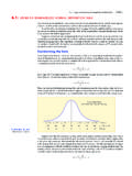
2 One rather obvious way to judge the near linearity of any plot is to compute its "correlation coefficient." When this is done for Normal Probability Plots , a formal test can be obtained that is essentially equivalent to the powerful Shapiro-Wilk test W and its approximation W. This note is basically an exposition of the utility of this simple yet powerful procedure. An Example Figure 1 shows a Normal Probability plot of 70 IQ scores that were obtained as a covariate in a study concerning the relative effectiveness of color versus black and white visual materials. This particular plot provides an example of the need for a simple objective way to assess the straightness of Probability Plots . This plot may seem curved enough at the ends to cast serious doubt upon the hypothesis on Normality . However, the "correlation coefficient" of this plot was , which is not significant at a = (critical value = ).
3 In fact, Plots as curved as this occur fairly often with Normal data (see, , [6]). Of course, there can still be practically significant departures from Normality , even though the hypothesis of Normality is not rejected. Figure 1: Normal Probability plot of IQ Scores of 70 Students + - - * - 2 - 2 3 + 2* - 3 - 4 - 23 - *3 + 3* - 22 - 22 - 4* - 3 + * 5 - 22 - 2 - 2* - * 3 + 2 - * - * - - +
4 +---------+---------+--------+---------+ ---------+ More Details A Normal Probability plot (see, , [6], [8], or [19]) is basically a plot of the ordered observations from a sample against the corresponding percentage points from the standard Normal distribution. If we denote the ordered observations in a sample of size n by {Yi}, then a Normal Probability plot can be produced by plotting the Yi on Normal " Probability " graph paper against some simple function like or pi . Using the special graph paper is equivalent to plotting the {Yi} on standard arithmetic graph paper against {bi} where bi is the pith percentage point of the standard Normal distribution. That is,. If the data come from a Normal distribution, they will fall on an approximately straight line, whereas if they come from some alternative distribution, the plot will exhibit some degree of curvature.
5 If the data fall nearly on a straight line, the "correlation coefficient" will be near unity, whereas if the plot is curved, the "correlation coefficient" will be smaller. If it falls below an appropriate critical value, doubt will be cast on the null hypothesis of Normality . Thus the " Probability plot correlation coefficient" version of the Shapiro-Wilk test is given by the familiar formula for a correlation coefficient, namely Since = 0, Rp can be simplified to , or where s2 denotes the sample variance. Filliben [9, 10] suggested plotted the {Yi} against {Ci} where Ci is the median of the ith order statistic in samples from the standard Normal distribution. The Ci may also be viewed as F-1(pi) where pi is the median of the ith order statistic in samples from the uniform distribution. For simplicity of computation, we suggest the use of pi or pi rather than pi since it does not appear to make any practical difference.
6 Either test has the highly desirable feature of linking together a graphical display of the data with a simple, objective test statistic. Some may object to the use of the term "correlation coefficient" since the {bi} are not random variables. However, another view is that, given any set of points in the plane, one can use the "correlation coefficient" associated with those points as a descriptive measure of how close they are to a straight line. In this sense, Rp can be thought of as a correlation coefficient. However, since Rp does not arise from sampling a bivariate distribution, it is not the same as the usual correlation coefficient. In fact, since both {bi} and {Yi} are ordered, Rp 0, and, in most practical cases, Rp is very large, even if the Yis come from a non- Normal population. A very useful approximation for making Probability Plots and/or computing Rp is [17, 12] A slightly more accurate approximation is [11] , where u = [-2 log e (p i )], and (g 0 , g 1.)
7 , g 5 ) = ( ; ; ; ; ; ). Either of these approximations is adequate. Use of these simple formulas in computer programs obviates the need to store the large tables of coefficients required for W and W. Relationship to Shapiro-Wilk and Shapiro-Francia Tests There is a very close relationship between R and the Shapiro-Wilk [16] test W and the Shapiro-Francia [15] approximation W. In fact, can be viewed as the "correlation coefficient" of a Probability plot in which the expected values of the standardized Normal order statistics mi are used as plotting positions rather than the Normal percentage points bi. Similarly, is proportional to the "correlation coefficient" associated with a Probability plot in which the plotting positions are the coefficients ai of the "best linear unbiased estimate" (BLUE) of the standard deviation.
8 Since the expected values of the Normal order statistics, the Normal percentage points and the (scaled) BLUE coefficients are all quite similar (see, , Table 1), similar properties should be expected among the three statistics W, W, and Rp. This indeed turns out to be the case as shown in the section entitled Power. Note in particular in Table 1 that the coefficients for W and Rp are in especially close agreement. The closeness of these three test statistics can also be anticipated from the theory of BLUEs and their approximations (see, , [7]). Table 1: Coefficients for the Three Tests W, W and Rp for n = 20. Test: Rp W W Coefficients Ratios i bi mi ai m i bi (ai ) bi 11. 12. 13. 14.
9 15. 16. 17. 18. 19. 20. Correlation between (all 20) bi and mi values = Correlation between (all 20) bi and ai values = Thus, Rp is basically a new way of viewing very good established procedures. Rp is easy to explain to students in an elementary statistics course and to researchers from other fields, since it is linked to a graphical technique ( Probability Plots ) and is based on a technique taught early in most courses (correlation coefficient). In addition, Rp is very easy to calculate, especially on a computer, since no special tables are required for its computation.
10 And the critical values needed to complete the test can be easily calculated using formula (1) in the section entitled Critical Values. For example, in Minitab [14] there is a command called NSCORES that computes the bi ( Normal scores) for any sample size. The following brief program reads in a batch of data, computes the Normal scores, does a Probability plot , and computes Rp. Note that no new commands need to be added to the system to compute Rp. SET THE FOLLOWING IQ SCORES INTO COLUMN C1 (data come here) NSCORES FOR DATA IN COL C1, PUT IN COL C2 plot COL C1 VS COL C2 ( Probability plot ) CORRELATION BETWEEN C1 AND C2 (R-SUB-P) STOP This program produced the plot in Figure 1. The critical importance of linking together graphical displays with objective test statistics cannot be overemphasized. This advantage is theoretically available with W and W but their use in this connection and their relationship with the "correlation coefficient" of Normal Probability Plots has not previously been noted.