Transcription of Potential Flow Theory - MIT
1 Hydrodynamics Reading #4. Hydrodynamics Prof. Techet Potential Flow Theory When a flow is both frictionless and irrotational, pleasant things happen. White, Fluid Mechanics 4th ed. We can treat external flows around bodies as invicid ( frictionless) and irrotational ( the fluid particles are not rotating). This is because the viscous effects are limited to a thin layer next to the body called the boundary layer. In graduate classes like , you'll learn how to solve for the invicid flow and then correct this within the boundary layer by considering viscosity. For now, let's just learn how to solve for the invicid flow. We can define a Potential function, ! ( x, z, t ) , as a continuous function that satisfies the basic laws of fluid mechanics: conservation of mass and momentum, assuming incompressible, inviscid and irrotational flow.
2 There is a vector identity (prove it for yourself!) that states for any scalar, " , " # "$ = 0. By definition, for irrotational flow, r ! " #V = 0. Therefore ! r V = "#. ! where ! = ! ( x, y, z , t ) is the velocity Potential function. Such that the components of velocity in Cartesian coordinates , as functions of space and time, are ! "! "! "! u= , v= and w = ( ). dx dy dz version updated 9/22/2005 -1- 2005 A. Techet Hydrodynamics Reading #4. laplace Equation The velocity must still satisfy the conservation of mass equation. We can substitute in the relationship between Potential and velocity and arrive at the laplace Equation, which we will revisit in our discussion on linear waves. !u + !v + !w = 0 ( ). !x !y !z " 2! " 2! " 2! + + =0 ( ). "x 2 "y 2 "z 2. LaplaceEquation " # 2! = 0. For your reference given below is the laplace equation in different coordinate systems: Cartesian, cylindrical and spherical .
3 Cartesian coordinates (x, y, z). r "# "# "# . V = ui + v j + wk = i + j + k = $#. "x "y "z $ 2# $ 2# $ 2#. 2. " #= 2 + 2 + 2 =0. $x $y $z ! Cylindrical coordinates ! (r, , z). r 2 = x 2 + y 2 , ! = tan "1 (y x ). r #$ 1 #$ #$. V = ur e r + u" e " + u z e z = e r + e " + e z = %$. #r r #" #z $ 2# 1 $# 1 $ 2# $ 2#. " 2# = 2. + + 2 2 + 2 =0. ! 14243 r $+. $ r r $ r $z 1 $ % $# (. 'r *. r $r & $r ). ! version updated 9/22/2005 -2- 2005 A. Techet Hydrodynamics Reading #4. spherical coordinates (r, , ). r 2 = x 2 + y 2 + z 2 , ! = cos "1 (x r ), or x = r cos ! , ! = tan "1 ( z y ). r $% 1 $% 1 $%. V = ur e r + u" e " + u# e # = e r + e " + e # = &%. $r r $" r sin " $#. $ 2# 2 $# 1 $ % $# ( 1 $ 2#. " 2# = 2. + + ' sin + * + =0. $r4. 1 r r 2 sin + $+ &. 2r4$3 $+ ) r 2 sin 2 + $, 2. ! 1 $ % 2 $# (. 'r *. r 2 $r & $r ).
4 ! Potential Lines Lines of constant ! are called Potential lines of the flow. In two dimensions #" #". d" = dx + dy #x #y d" = udx + vdy Since d" = 0 along a Potential line, we have ! dy u =" ( ). dx v ! dy v Recall that streamlines are lines !everywhere tangent to the velocity, = , so Potential dx u lines are perpendicular to the streamlines. For inviscid and irrotational flow is indeed quite pleasant to use Potential function, ! , to represent the velocity field, as it reduced the problem from having three unknowns (u, v, w) to only one unknown ( ! ). ! As a point to note here, many texts use stream function instead of Potential function as it is slightly more intuitive to consider a line that is everywhere tangent to the velocity. Streamline function is represented by ! . Lines of constant ! are perpendicular to lines of constant !
5 , except at a stagnation point. version updated 9/22/2005 -3- 2005 A. Techet Hydrodynamics Reading #4. Luckily ! and ! are related mathematically through the velocity components: #! #". u= = ( ). #x #y #! #". v= =$ ( ). #y #x equations ( ) and ( ) are known as the Cauchy-Riemann equations which appear in complex variable math (such as ). Bernoulli Equation The Bernoulli equation is the most widely used equation in fluid mechanics, and assumes frictionless flow with no work or heat transfer. However, flow may or may not be irrotational. When flow is irrotational it reduces nicely using the Potential function in place of the velocity vector. The Potential function can be substituted into equation resulting in the unsteady Bernoulli Equation. ! # $" + 1 ($" )2 + $p + ! g $z = 0. { } ( ). #t 2. or {. $ ". #!}
6 1. #t 2 }. + "V 2 + p + " gz = 0 . ( ). + "V 2 + p + " gz = c(t ). #! 1. UnsteadyBernoulli $ " ( ). #t 2. version updated 9/22/2005 -4- 2005 A. Techet Hydrodynamics Reading #4. Summary Potential Stream Function v Definition V = "! V = " #! Continuity " 2! = 0 Automatically Satisfied (! " V = 0 ). Irrotationality Automatically Satisfied v v v " # (" #! ) = " (" $! ) % " 2! = 0. (! " V = 0 ). ! In 2D : w = 0, =0. !z v " 2! = 0 for continuity ! " ! z # 2! = 0 for irrotationality Cauchy-Riemann equations for ! and ! from complex analysis: # = ! + i" , where ! is real part and ! is the imaginary part Cartesian (x, y) "! "! u= u=. "x "y "! "! v= v=#. "y "x Polar (r, ) "! 1 #! u= u=. "r r #". 1 #! "! v= v=#. r #" "r For irrotational flow use: ! For incompressible flow use: ! For incompressible and irrotational flow use: !
7 And ! version updated 9/22/2005 -5- 2005 A. Techet Hydrodynamics Reading #4. Potential flows Potential functions ! (and stream functions,! ) can be defined for various simple flows. These Potential functions can also be superimposed with other Potential functions to create more complex flows. Uniform, Free Stream Flow (1D). r V = Ui + 0 j + 0 k ( ). #! #". u =U = = ( ). ! #x #y #! #". v=0= =$ ( ). #y #x We can integrate these expressions, ignoring the constant of integration which ultimately does not affect the velocity field, resulting in ! and ! ! = Ux and ! = Uy ( ). Therefore we see that streamlines are horizontal straight lines for all values of y (tangent everywhere to the velocity!) and that equipotential lines are vertical straight lines perpendicular to the streamlines (and the velocity!) as anticipated.
8 2D Uniform Flow: V = (U , V , 0) ; ! = Ux + Vy ; ! = Uy " Vx 3D Uniform Flow: V = (U , V , W ) ; ! = Ux + Vy + Wz ; no stream function in 3D. version updated 9/22/2005 -6- 2005 A. Techet Hydrodynamics Reading #4. Line Source or Sink Consider the z-axis (into the page) as a porous hose with fluid radiating outwards or being drawn in through the pores. Fluid is flowing at a rate Q (positive or outwards for a source, negative or inwards for a sink) for the entire length of hose, b. For simplicity take a unit length into the page (b = 1) essentially considering this as 2D flow. Polar coordinates come in quite handy here. The source is located at the origin of the coordinate system. From the sketch above you can see that there is no circumferential velocity, but only radial velocity. Thus the velocity vector is r V = ur e r + u" e " + u z e z = ur e r + 0 e " + 0 e z ( ).
9 Q m #$ 1 #%. ur = = = = ( ). 2 "r r #r r #&. ! and 1 #$ #&. ! u" = 0 = =% ( ). r #" #r Integrating the velocity we can solve for ! and ! ! ! = m ln r and ! = m" ( ). Q. where m = . Note that ! satisfies the laplace equation except at the origin: 2! r = x 2 + y 2 = 0 , so we consider the origin a singularity (mathematically speaking) and exclude it from the flow. The net outward volume flux can be found by integrating in a closed contour around the origin of the source (sink): 2! % V # n dS = %% $ # V dS = %. C S. o ur r d" = Q. version updated 9/22/2005 -7- 2005 A. Techet Hydrodynamics Reading #4. Irrotational Vortex (Free Vortex). A free or Potential vortex is a flow with circular paths around a central point such that the velocity distribution still satisfies the irrotational condition ( the fluid particles do not themselves rotate but instead simply move on a circular path).
10 See figure 2. Figure 2: Potential vortex with flow in circular patterns around the center. Here there is no radial velocity and the individual particles do not rotate about their own centers. It is easier to consider a cylindrical coordinate system than a Cartesian coordinate system with velocity vector V = (ur , u! , u z ) when discussing point vortices in a local reference frame. For a 2D vortex, u z = 0 . Referring to figure 2, it is clear that there is also no radial velocity. Thus, r V = ur e r + u" e " + u z e z = 0 e r + u" e " + 0 e z ( ). where "# 1 "$. ! ur = 0 = = ( ). "r r "%. and 1 #$ #&. ! u" = ? = =% . ( ). r #" #r Let us derive u" . Since the flow is considered irrotational, all components of the vorticity vector must be zero. The vorticity in cylindrical coordinates is ! # 1 "u z "u! $ # "u "u $ # 1 "ru!