Transcription of Spatial Resolution
1 423 CHAPTER25 Special Imaging TechniquesThis chapter presents four specific aspects of image processing . First, ways to characterize thespatial Resolution are discussed. This describes the minimum size an object must be to be seenin an image . Second, the signal-to-noise ratio is examined, explaining how faint an object canbe and still be detected. Third, morphological techniques are introduced. These are nonlinearoperations used to manipulate binary images (where each pixel is either black or white). Fourth,the remarkable technique of computed tomography is described. This has revolutionized medicaldiagnosis by providing detailed images of the interior of the human body. Spatial ResolutionSuppose we want to compare two imaging systems, with the goal ofdetermining which has the best Spatial Resolution .
2 In other words, we want toknow which system can detect the smallest object. To simplify things, wewould like the answer to be a single number for each system. This allows adirect comparison upon which to base design decisions. Unfortunately, a singleparameter is not always sufficient to characterize all the subtle aspects ofimaging. This is complicated by the fact that Spatial Resolution is limited bytwo distinct but interrelated effects: sample spacing and sampling aperturesize. This section contains two main topics: (1) how a single parameter canbest be used to characterize Spatial Resolution , and (2) the relationship betweensample spacing and sampling aperture size.
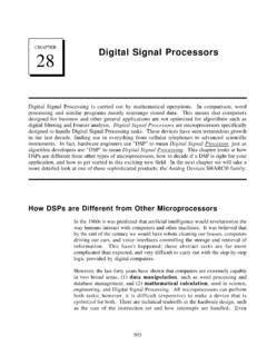
3 Figure 25-1a shows profiles from three circularly symmetric PSFs: thepillbox, the Gaussian, and the exponential. These are representative of thePSFs commonly found in imaging systems. As described in the last chapter,the pillbox can result from an improperly focused lens system. Likewise,the Gaussian is formed when random errors are combined, such as viewingstars through a turbulent atmosphere. An exponential PSF is generatedwhen electrons or x-rays strike a phosphor layer and are converted intoThe Scientist and Engineer's Guide to Digital Signal PSFS patial frequency (lp per unit distance) MTFFIGURE 25-1 FWHM versus MTF. Figure (a) shows profiles of three PSFs commonly found in imaging systems: (P) pillbox,(G) Gaussian, and (E) exponential.
4 Each of these has a FWHM of one unit. The corresponding MTFs areshown in (b). Unfortunately, similar values of FWHM do not correspond to similar MTF This is used in radiation detectors, night vision light amplifiers, and CRTdisplays. The exact shape of these three PSFs is not important for thisdiscussion, only that they broadly represent the PSFs seen in real worldapplications. The PSF contains complete information about the Spatial Resolution . To expressthe Spatial Resolution by a single number, we can ignore the shape of the PSFand simply measure its width. The most common way to specify this is by theFull-Width-at-Half-Maximum (FWHM) value. For example, all the PSFs in(a) have an FWHM of 1 unit. Unfortunately, this method has two significant drawbacks.
5 First, it does notmatch other measures of Spatial Resolution , including the subjective judgementof observers viewing the images. Second, it is usually very difficult to directlymeasure the PSF. Imagine feeding an impulse into an imaging system; that is,taking an image of a very small white dot on a black background. Bydefinition, the acquired image will be the PSF of the system. The problem is,the measured PSF will only contain a few pixels, and its contrast will be you are very careful, random noise will swamp the measurement. Forinstance, imagine that the impulse image is a 512 512 array of all zeros exceptfor a single pixel having a value of 255. Now compare this to a normal imagewhere all of the 512 512 pixels have an average value of about 128.
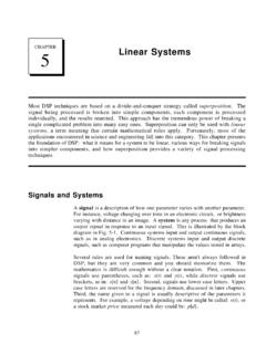
6 In looseterms, the signal in the impulse image is about 100,000 times weaker than anormal image . No wonder the signal-to-noise ratio will be bad; there's hardlyany signal! A basic theme throughout this book is that signals should be understood in thedomain where the information is encoded. For instance, audio signals shouldbe dealt with in the frequency domain, while image signals should be handledin the Spatial domain. In spite of this, one way to measure image Resolution isby looking at the frequency response. This goes against the fundamentalChapter 25- Special Imaging Techniques425 Pixel number060120180240050100150200250 Pixel number060120180240050100150200250a. Example profile at 12 lp/mmb. Example profile at 3 lp/mm402010521530743 FIGURE 25-2 Line pair gauge.
7 The line pair gauge isa tool used to measure the Resolution ofimaging systems. A series of black andwhite ribs move together, creating acontinuum of Spatial frequencies. Theresolution of a system is taken as thefrequency where the eye can no longerdistinguish the individual ribs. Thisexample line pair gauge is shownseveral times larger than the calibratedscale indicates. line pairs / mmPixel valuePixel valuephilosophy of this book; however, it is a common method and you need tobecome familiar with it. Taking the two-dimensional Fourier transform of the PSF provides the two-dimensional frequency response. If the PSF is circularly symmetric, itsfrequency response will also be circularly symmetric. In this case, completeinformation about the frequency response is contained in its profile.
8 That is,after calculating the frequency domain via the FFT method, columns 0 to N/2in row 0 are all that is needed. In imaging jargon, this display of the frequencyresponse is called the Modulation Transfer Function (MTF). Figure 25-1bshows the MTFs for the three PSFs in (a). In cases where the PSF is notcircularly symmetric, the entire two-dimensional frequency response containsinformation. However, it is usually sufficient to know the MTF curves in thevertical and horizontal directions ( , columns 0 to N/2 in row 0, and rows 0to N/2 in column 0). Take note: this procedure of extracting a row or columnfrom the two-dimensional frequency spectrum is not equivalent to taking theone-dimensional FFT of the profiles shown in (a).
9 We will come back to thisissue shortly. As shown in Fig. 25-1, similar values of FWHM do notcorrespond to similar MTF 25-2 shows a line pair gauge, a device used to measure imageresolution via the MTF. Line pair gauges come in different forms dependingon the particular application. For example, the black and white pattern shownin this figure could be directly used to test video cameras. For an x-rayimaging system, the ribs might be made from lead, with an x-ray transparentmaterial between. The key feature is that the black and white lines have acloser spacing toward one end. When an image is taken of a line pair gauge,the lines at the closely spaced end will be blurred together, while at the otherend they will be distinct.
10 Somewhere in the middle the lines will be just barelyseparable. An observer looks at the image , identifies this location, and readsthe corresponding Resolution on the calibrated scale. The Scientist and Engineer's Guide to Digital Signal Processing426 The way that the ribs blur together is important in understanding thelimitations of this measurement. Imagine acquiring an image of the linepair gauge in Fig. 25-2. Figures (a) and (b) show examples of the profilesat low and high Spatial frequencies. At the low frequency, shown in (b),the curve is flat on the top and bottom, but the edges are blurred, At thehigher Spatial frequency, (a), the amplitude of the modulation has beenreduced. This is exactly what the MTF curve in Fig.