Transcription of Speech Recognition Using Deep Learning Algorithms
1 Speech Recognition Using Deep Learning Algorithms Yan Zhang, SUNet ID: yzhang5 Instructor: Andrew Ng Abstract: Automatic Speech Recognition , translating of spoken words into text, is still a challenging task due to the high viability in Speech signals. Deep Learning , sometimes referred as representation Learning or unsupervised feature Learning , is a new area of machine Learning . Deep Learning is becoming a mainstream technology for Speech Recognition and has successfully replaced Gaussian mixtures for Speech Recognition and feature coding at an increasingly larger scale. The main target of this course project is to applying typical deep Learning Algorithms , including deep neural networks (DNN) and deep belief networks (DBN), for automatic continuous Speech Recognition . 1. introduction Automatic Speech Recognition , translating of spoken words into text, is still a challenging task due to the high viability in Speech signals.
2 For example, speakers may have different accents, dialects, or pronunciations, and speak in different styles, at different rates, and in different emotional states. The presence of environmental noise, reverberation, different microphones and recording devices results in additional variability. Conventional Speech Recognition systems utilize Gaussian mixture model (GMM) based hidden Markov models (HMMs) [1, 2] to represent the sequential structure of Speech signals. HMMs are used in Speech Recognition because a Speech signal can be viewed as a piecewise stationary signal or a short-time stationary signal. In a short time-scale, Speech can be approximated as a stationary process. Speech can be thought of as a Markov model for many stochastic , each HMM state utilizes a mixture of Gaussian to model a spectral representation of the sound wave.
3 HMMs-based Speech Recognition systems can be trained automatically and are simple and computationally feasible to use. However, one of the main drawbacks of Gaussian mixture models is that they are statistically inefficient for modeling data that lie on or near a non-linear manifold in the data space. Neural networks trained by back-propagation error derivatives emerged as an attractive acoustic modeling approach for Speech Recognition in the late 1980s. In contrast to HMMs, neural networks make no assumptions about feature statistical properties. When used to estimate the probabilities of a Speech feature segment, neural networks allow discriminative training in a natural and efficient manner. However, in spite of their effectiveness in classifying short-time units such as individual phones and isolated words, neural networks are rarely successful for continuous Recognition tasks, largely because of their lack of ability to model temporal dependencies.
4 Thus, one alternative approach is to use neural networks as a pre-processing feature transformation, dimensionality reduction for the HMM based Recognition . Deep Learning [6 -9], sometimes referred as representation Learning or unsupervised feature Learning , is a new area of machine Learning . Deep Learning is becoming a mainstream technology for Speech Recognition [10-17] and has successfully replaced Gaussian mixtures for Speech Recognition and feature coding at an increasingly larger scale. In the course project, we focus on deep belief networks (DBNs) for Speech Recognition . The main goal of this course project can be summarized as: 1) Familiar with end-to -end Speech Recognition process. 2) Review state-of-the-art Speech Recognition techniques. 3) Learn and understand deep Learning Algorithms , including deep neural networks (DNN), deep belief networks (DBN), and deep auto-encoders (DAE).
5 4) Applying deep Learning Algorithms to Speech Recognition and compare the Speech Recognition performance with conventional GMM-HMM based Speech Recognition method. Feature ExtractionSpeech SignalDecoderRecognized WordsAcousticModelsPronunciationDictiona ryLanguageModels Fig. 1 A typical system architecture for automatic Speech Recognition 2. Automatic Speech Recognition System Model The principal components of a large vocabulary continuous Speech recognizer [1] [2] are illustrated in Fig. 1. The input audio waveform from a microphone is converted into a sequence of fixed size acoustic vectors =[ 1, , ]. This process is called feature extraction. The decoder then attempts to find the sequence of words =[ 1, , ] which is most likely to have generated , the decoder tries to find = { ( | )} However, since ( | ) is difficult to model directly, Bayes Rule is used to transform the above equation into the equivalent problem of finding: = { ( | ) ( )} The likelihood ( | ) is determined by an acoustic model and the prior ( ) is determined by a language model.
6 For any given , the corresponding acoustic model is synthesized by concatenating phone models to make words as defined by a pronunciation dictionary. The parameters of these phone models are estimated from training data consisting of Speech waveforms and their orthographic transcriptions. The language model is typically an -gram model in which the probability of each word is conditioned only on its 1 predecessors. The N-gram parameters are estimated by counting N-tuples in appropriate text corpora. The decoder operates by searching through all possible word sequences Using pruning to remove unlikely hypotheses thereby keeping the search tractable. When the end of the utterance is reached, the most likely word sequence is output. Alternatively, modern decoders can generate lattices containing a compact representation of the most likely hypotheses.
7 A. Feature Extraction In automatic Speech Recognition , it is common to extract a set of features from Speech signal. Classification is carried out on the set of features instead of the Speech signals themselves. The feature extraction stage seeks to provide a compact representation of the Speech waveform. This form should minimise the loss of information that discriminates between words, and provide a good match with the distributional assumptions made by the acoustic models. A popular feature vector Mel-frequency cepstral coefficients (MFCC), which provides a compact Speech signal representation that are the results of a cosine transform of the real logarithm of the short-term energy spectrum expressed on a mel-frequency scale. MFCC coefficients are generated by applying a truncated discrete cosine transformation (DCT) to a log spectral estimate computed by smoothing an FFT with around 20 frequency bins distributed non-linearly across the Speech spectrum.
8 The nonlinear frequency scale used is called a mel scale and it approximates the response of the human ear. The DCT is applied in order to smooth the spectral estimate and approximately decorrelate the feature elements. After the cosine transform the first element represents the average of the log-energy of the frequency bins. This is sometimes replaced by the log-energy of the frame, or removed completely. b. Hidden Markov Models Predominantly, HMMs are used in ASR. A HMM is a stochastic finite state automaton built from a finite set of possible states ={ 1, , } with instantaneous transitions with certain probabilities between these states. Each of these states is associated with a specific emission probability distribution ( | ). Thus, HMMs can be used to model a sequence X of feature vectors as a piecewise stationary process where each stationary segment is associated with a specific HMM state.
9 This approach defines two concurrent stochastic processes: the sequence of HMM-states modeling the temporal dynamics of Speech , and a set of state output processes modeling the locally stationary property of the Speech signal. In Speech Recognition , we have to find the HMM which maximizes the posterior probability ( | ) of the hypothesized HMM given a sequence X of feature-vectors. Since this probability cannot be computed directly, it is usually split Using Bayes rule into the acoustic model (likelihood) ( | ) and a prior ( ) representing the language model: ( | ) ( | ) ( ). : The DBN is composed of RBMs. 3. Deep Belief Networks Deep Belief Networks (DBNs) are neural networks consisting of a stack of restricted Boltzmann machine (RBM) layers that are trained one at a time, in an unsupervised fashion to induce increasingly abstract representations of the inputs in subsequent layers.
10 Restricted Boltzmann Machines (RBMs) and Training As shown in Fig. 2 (a), Each RBM has an input layer (visible layer) and a hidden layer of stochastic binary units. Visible and hidden layers are connected with a weight matrix and no connections exist between units in the same layer. Signal propagation can occur in two ways: Recognition , where visible activations propagate to the hidden units; and reconstruction, where hidden activations propagate to visible units. The same weight matrix (transposed) is used for both Recognition and reconstruction. By minimizing the difference between the original input and its reconstruction ( reconstruction error) through a procedure called contrastive divergence (CD), the weights can be trained to generate the input patterns presented to the RBM with high probability.