Transcription of Switch-mode power converter compensatin made easy
1 Switch-mode power converter compensation made easyRobert SheehanSystems Manager, power Design ServicesMember Group Technical StaffLouis DianaField Application,America Sales and MarketingSenior Member Technical StaffTexas InstrumentsTexas Instruments 2 September 2016 IntroductionA Switch-mode power supply (SMPS) regulates the output voltage against any changes in output loading or input line voltage. An SMPS accomplishes this regulation with a feedback loop, which requires compensation if it has an error amplifier with linear feedback. This paper covers the necessary definitions and theory required to understand how a linear feedback loop works. We will define poles and zeros and power - stage characteristics, along with various error amplifiers; discuss isolated feedback and optocouplers; and give examples of how to compensate various buck, boost and buck-boost topologies.
2 We will cover voltage-mode control and current-mode control methods. Unless otherwise noted, equations and graphs depict fixed-frequency, continuous-conduction-mode (CCM) operation. We will define discontinuous-conduction-mode (DCM) versus CCM, and how each affects the feedback loop. This paper also includes a section on the practical limits of devices used in SMPS designers would appreciate a how-to reference paper that they can use to look up compensation solutions to various topologies with various feedback modes. We are striving to provide this in a single and compensation definitionsAs stated previously, a SMPS s primary function is to regulate its output against input/output variations and transients, which requires a feedback loop. Figure 1 shows a typical SMPS with a feedback 1. A test signal injected into the feedback of the control loop measures the frequency this paper as a quick look-up reference can help designers compensate the most popular Switch-mode power converter have been designing Switch-mode power converters for some time now.
3 If you re new to the design field or you don t compensate converters all the time, compensation requires some research to do correctly. This paper will break the procedure down into a step-by-step process that you can follow to compensate a power will explain the theory of compensation and why it is necessary, examine various power stages, and show how to determine where to place the poles and zeros of the compensation network to compensate a power converter . We will examine typical error amplifiers as well as transconductance amplifiers to see how each affects the control loop and work through a number of topologies/examples so that power engineers have a quick reference when they need to compensate a power 1 Texas Instruments 3 September 2016 Figure 1 contains a power stage and an error amplifier. The power stage contains all of the magnetics and power switches, as well as a pulse-width modulated (PWM) controller.
4 The error amplifier provides the feedback mechanism and compensation. A voltage divider connected to the output provides a sample of the output voltage, which is compared to a reference voltage by the error amplifier. The error voltage coming out of the error amplifier drives the PWM duty cycle higher if the output voltage is low, or drives the PWM duty cycle lower if the output voltage is high. Thus, the feedback scheme used here is negative feedback. Loop gain is the gain around the feedback loop, comprising the product of error-amplifier gain, modulator gain and power - stage gain. The feedback loop s gain and phase response versus frequency will determine how well the SMPS will bandwidth of the control loop determines its speed in responding to a transient condition. Compensation adjusts the loop bandwidth and tailors the frequency response. Increasing the loop bandwidth increases the speed at which the SMPS reacts to a transient.
5 Therefore, maximizing the crossover frequency will produce a quicker transient margin, which we discuss in the next section, also plays an important role in compensation. Figure 2 shows the results of low phase margin. In this case there is ringing after the load transient and the loop is underdamped. This is not a desirable Figure 3, the phase margin has increased; therefore, the waveform does not show any ringing after the load transient. This response is well damped. Figure 2:.Poor transient response characterized by underdamped ringing of the output voltage when stepping the load 3. Good transient response exhibits no ringing with a critically damped and gain-margin definitionsPhase and gain margin are parameters used to identify the health of a feedback loop. A control loop is unstable if the loop has unity gain when the phase passes through zero. Gain margin is the gain value when the phase passes through 0 degrees.
6 This is measured in decibels and should be a negative number. Phase margin is the value of the phase measured in degrees when the gain passes through zero. This is measured in degrees and should be a positive number (Figure 4).Figure 2 VOUTIOUTF igure 3 VOUTIOUTT exas Instruments 4 September 2016 Figure 4. Phase margin is the difference in degrees when the gain crosses zero. Gain margin is the difference in decibels when the phase crosses phase margin is required to prevent oscillations. A phase margin of 45 degrees or greater is the design goal. A gain margin of 6 dB is the minimum, while 10 dB is considered higher crossovers are generally preferable, there are practical limitations. The rule of thumb is one-fifth to one-tenth the switching frequency. Attenuation at the switching frequency is also important for noise immunity to minimize jitter. The gain should ideally pass through zero with a slope of 20 dB/decade.
7 This will maximize gain margin and will also negate the chance of the gain turning positive at a higher frequency where the phase may be going through zero. If that happens, you could have an unstable control and zeros definitionsEquation 1 defines a pole where s is in the denominator. At the frequency of the pole the gain is 3 dB down and rolling off at a 20 dB/decade slope. The phase starts to decrease one decade before the pole frequency, is 45 degrees down at the pole frequency, and continues to decrease another 45 degrees for one more decade. The total change is 90 degrees over two decades (Figure 5). (1) Figure 5. The Bode plot of a pole shows the gain decreasing by 20 dB/decade, with a phase shift at higher frequencies of 90 2 defines a zero where s is in the numerator. At the frequency of the zero the gain is 3 dB up and increasing at a +20 dB/decade slope.
8 The phase starts to increase one decade before the zero frequency, is 45 degrees up at the zero frequency, and continues to increase another 45 degrees for one more decade. The total change is 90 degrees over two decades (Figure 6). (2) Figure 6. The Bode plot of a zero shows the gain increasing by +20 dB/decade, with a phase shift at higher frequencies of +90 7 shows an inverted zero often used with a low-frequency pole when using the mid-band gain as the reference gain, defined by Equation 3. The inverted zero still has s in the numerator, but s and are 110 100 1000 Phase ( )Magnitude (dB)Frequency (kHz)Control Loop Frequency ResponsePhasemarginGain margin PssH +=11)(Figure 1 10 100 1000 Phase ( )Magnitude (dB)Frequency (kHz) 11)(ZssH +=Figure 1 10 100 1000 Phase ( )Magnitude (dB)Frequency (kHz)Texas Instruments 5 September 2016 (3) Figure 7.
9 The Bode plot of an inverted zero shows the gain going up and to the left of the reference gain, shown here as 0 dB. This cancels a pole at some lower frequency so that the phase changes from 90 degrees to 0 right-half-plane zero is characteristic of boost and buck-boost power stages. The magnitude increases at 20 dB/decade with an associated phase lag of 90 degrees. As you can see in Equation 4, s is in the numerator, but it is negative. This makes compensating the converter more difficult (Figure 8). (4) Figure 8. The Bode plot of a right-half-plane zero shows the gain increasing by +20 dB/decade, with a phase shift at higher frequencies of 90 mentioned in the introduction, we will discuss two types of loop control methods: voltage-mode control and current-mode control. The control method determines the characteristics of the of the power stage . For example, in a voltage-mode buck converter the inductor-capacitor (LC) filter exhibits a complex conjugate pole at the LC resonant frequency.
10 This means that there are two poles at the same frequency, and the gain changes 40 dB/decade with an associated phase change of 180 degrees. A current-mode buck converter does not have a complex pole at the LC resonant 5 shows the transfer function of a complex conjugate pole with a quality factor, Q, associated with the LC filter. Q is a measure of the sensitivity or quality of the tuned circuit. A higher Q value corresponds to a narrower bandwidth of the tuned circuit. A high Q value is not so good for a power -supply output filter, however, because as Q increases the phase slope increases. This means that the phase changes much more quickly over a small band of frequencies, whereas two regular poles would change with a more gradual slope over two decades. (5)Figure 9 illustrates how phase slope increases as Q increases. Since a high Q LC filter can cause a 180 degree phase shift in the loop Bode plot, it is important to understand the Q of the LC filter in order to compensate for this phase change.