The Box-Jenkins Method

1 NCSS Statistical Software 470-1 NCSS, LLC. All Rights Reserved. Chapter 470 The Box-Jenkins Method Introduction Box - Jenkins Analysis refers to a systematic Method of identifying, fitting, checking, and using integrated autoregressive, moving average (ARIMA) time series models. The Method is appropriate for time series of medium to long length (at least 50 observations). In this chapter we will present an overview of the Box-Jenkins Method , concentrating on the how-to parts rather than on the theory. Most of what is presented here is summarized from the landmark book on time series analysis written by George Box and Gwilym Jenkins (1976). A time series is a set of values observed sequentially through time. The series may be denoted by XXXt12,,, , where t refers to the time period and X refers to the value.

2 If the X s are exactly determined by a mathematical formula, the series is said to be deterministic. If future values can be described only by their probability distribution, the series is said to be a statistical or stochastic process. A special class of stochastic processes is a stationary stochastic process. A statistical process is stationary if the probability distribution is the same for all starting values of t. This implies that the mean and variance are constant for all values of t. A series that exhibits a simple trend is not stationary because the values of the series depend on t. A stationary stochastic process is completely defined by its mean, variance, and autocorrelation function. One of the steps in the Box - Jenkins Method is to transform a non-stationary series into a stationary one.

3 Autocorrelation Function The stationary assumption allows us to make simple statements about the correlation between two successive values, Xt and Xtk+. This correlation is called the autocorrelation of lag k of the series. The autocorrelation function displays the autocorrelation on the vertical axis for successive values of k on the horizontal axis. The following figure shows the autocorrelation function of the sunspot data. NCSS Statistical Software The Box-Jenkins Method 470-2 NCSS, LLC. All Rights Reserved. Since a stationary series is completely specified by its mean, variance, and autocorrelation function, one of the major (and most subjective) tasks in Box-Jenkins analysis is to identify an appropriate model from the sample autocorrelation function. Although the sample autocorrelations contains random fluctuations, for moderate sample sizes they are fairly accurate in signaling the order of the ARIMA model .

4 The ARMA model The ARMA (autoregressive, moving average) model is defined as follows: XXXaaattptpttqtq=+ ++ 1111 where the 's(phis) are the autoregressive parameters to be estimated, the 's (thetas) are the moving average parameters to be estimated, the X s are the original series, and the a s are a series of unknown random errors (or residuals) which are assumed to follow the normal probability distribution. Box-Jenkins use the backshift operator to make writing these models easier. The backshift operator, B, has the effect of changing time period t to time period t-1. Thus BXXtt= 1and BXXtt22= . Using this backshift notation, the above model may be rewritten as: ()()1111 = BBXBB apptqqt This may be abbreviated even further by writing: ()() ptqtBXB a= where ()() pppBBB= 11 and ()() qqqBBB= 11 NCSS Statistical Software The Box-Jenkins Method 470-3 NCSS, LLC.

5 All Rights Reserved. These formulas show that the operators () pBand () qBare polynomials in B of orders p and q respectively. One of the benefits of writing models in this fashion is that we can see why several models may be equivalent. For example, consider the model XXXattttt= + 0 80 150 This could be rewritten in the form of ( ) as: ()()10 80 1510 32 += ..BBXB att Notice that the polynomial on the left may be factored, so that we can rewrite the model as ()()()10 510 310 3 = ..BBXB att Finally, canceling the (1 - ) from both sides leaves the simpler, but equivalent, model ()10 5 =.BXatt or XXattt=+ 0 51. Note that this is a much simpler model ! This type of model rearrangement is used by experienced Box-Jenkins forecasters to obtain the simplest models possible. The Theoretical ARIMA program displays the roots of the two polynomials, () pBand () qB, so you can see possible model simplifications.

6 Nonstationary Models Many time series encountered in practice exhibit nonstationary behavior. Usually, the nonstationarity is due to a trend, a change in the local mean, or seasonal variation. Since the Box-Jenkins methodology is for stationary models only, we have to make some adjustments before we can model these nonstationary series. We use one of two methods for reducing a nonstationary series with trend to a stationary series (without trend): 1. Use the first differences of the series, WXXttt= 1. Note that this can be rewritten as ()WBXtt= 1. A more general form of this equation is: ()()() pdtqtBBXB a1 = where d is the order of differencing. This is known as the ARIMA(p,d,q) model . 2. Fit a least squares trend and fit the Box-Jenkins model to the residuals. If the model exhibits an occasional change of mean, first differences will result in a stationary model .

7 For seasonal series, Box-Jenkins provided a modification to this equation that will be the subject of the next section. NCSS Statistical Software The Box-Jenkins Method 470-4 NCSS, LLC. All Rights Reserved. Seasonal Time Series To deal with series containing seasonal fluctuations, Box-Jenkins recommend the following general model : ()()()()()() pPdsDtqQstBBBBXBBa 11 = where d is the order of differencing, s is the number of seasons per year, and D is the order of seasonal differencing. The operator polynomials are ()() pppBBB= 11 ()() qqqBBB= 11 ()() PsspspBBB= 11 ()() QssQsQBBB= 11 Note that ()1 = BXXX sttts. Box-Jenkins explain that the maximum value of d, D, p, q, P, and Q is two. Hence, these operator polynomials are usually simple expressions.

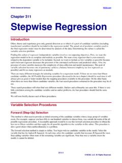
8 Partial Autocorrelation Function We previously discussed the autocorrelation function, which gives the correlations between different lags of a series. The Partial Autocorrelation Function is a second function that expresses information useful in determining the order of an ARIMA model . This function is constructed by calculating the partial correlation betweenXtandXt 1, XtandXt 2, and so on, statistically adjusting out the influence of intermediate lags. For example, the partial autocorrelation of lag four is the partial correlation betweenXtand Xt 4after statistically removing the influence of Xt 1,Xt 2, andXt 3from bothXtandXt 4. The autoregressive order, p, is estimated as the lag of the last large partial autocorrelation. For example, suppose the partial autocorrelations were Lag Partial Autocorrelation 1 2 3 4 5 6 7 We would conclude that a reasonable value for p is four, since the partial autocorrelations are relatively small after the fourth lag.

9 NCSS Statistical Software The Box-Jenkins Method 470-5 NCSS, LLC. All Rights Reserved. Box-Jenkins Methodology An Overview The Box-Jenkins Method refers to the iterative application of the following three steps: 1. Identification. Using plots of the data, autocorrelations, partial autocorrelations, and other information, a class of simple ARIMA models is selected. This amounts to estimating appropriate values for p, d, and q. 2. Estimation. The phis and thetas of the selected model are estimated using maximum likelihood techniques, backcasting, etc., as outlined in Box-Jenkins (1976). 3. Diagnostic Checking. The fitted model is checked for inadequacies by considering the autocorrelations of the residual series (the series of residual, or error, values). These steps are applied iteratively until step three does not produce any improvement in the model .

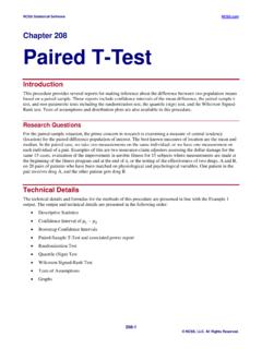
10 We will now go over these steps in detail. model Identification Assuming for the moment that there is no seasonal variation, the objective of the model identification step is to select values of d and then p and q in the ARIMA(p,d,q) model . When the series exhibits a trend, we may either fit and remove a deterministic trend or difference the series. Box-Jenkins seem to prefer differencing, while several other authors prefer the deterministic trend removal. The first step, in either case, is to look at the plots of the autocorrelations and partial autocorrelations. A series with a trend will have an autocorrelation patterns similar to the following: We notice that the large autocorrelations persist even after several lags. This indicates that either a trend should be removed or that the series should be differenced.