Transcription of The P/B-ROE Model Revisited
1 The P/B-ROE Model Revisited Jarrod Wilcox Wilcox Investment Inc &. Thomas Philips Paradigm Asset Management Agenda Characterizing a good equity Model : Its virtues and uses Static vs. dynamic models The P/B-ROE Model : Closed form & approximate solutions Cross-sectional explanation using the P/B-ROE Model Cross-sectional prediction using the P/B-ROE Model Time-series explanation using the P/B-ROE Model Time-series prediction using the P/B-ROE Model 2. What Characterizes a Good Model ? Economic realism in its intellectual underpinnings Must be grounded in a realistic view of the firm Must allow the incorporation of economic constraints Earnings cannot grow faster than revenues in perpetuity Parsimony and computability Should require relatively few inputs Inputs should be readily available or easily estimated from data Widespread applicability Model prices should explain prevailing prices without significant bias Model residuals should predict future returns Should be applicable in cross-section and time-series 3.
2 Who Might Use a Good Model ? Corporate officers If the Model can guide them on how best to increase firm value Fundamental analysts If the Model can help them better evaluate a firm and its management Investment bankers and buyers and sellers of companies If the Model can generate unbiased valuations Investors If the Model 's residuals are predictive of future returns 4. Models in Widespread Use Today . E[ FCFi ]. Dividend Discount Model ( Williams, 1938): P0 = . i =1 (1 + k )i Intellectual root of almost all models in use today Free Cash Flow1. Gordon Growth Model (1962): P =. k g Free cash flows grow at a constant rate in perpetuity . E[(ri k ) Bi 1 ]. Edward-Bell-Ohlson Equation (1961): P = B0 + . i =1 (1 + k )i Apply clean surplus relationship to DDM and rearrange terms Various multi-stage versions of the DDM.
3 3 stages Model growth, steady state and decline 5. Static vs. Dynamic Models A static Model evaluates price at a point in time Estimate inputs at fixed points in time, discount back to get today's price Examples: DDM, EBO. A dynamic Model evolves some function of price over time Some evolve price, others evolve a valuation ratio Trajectory must be consistent with the Model : a hint of continuous time Examples: Options (Black-Scholes), pricing a zero-coupon bond Bond price trajectory must be consistent with the yield curve Both static and dynamic models can have the same intellectual roots Both ultimately give us a fix on today's price Choice of one over the other is empirical which works better in practice 6. A Brief History of Dynamic Models Jarrod Wilcox (FAJ 1984): P/B-ROE Model .
4 Two stage growth Model ,with first phase ending at time T. Determine the trajectory of P/B subject to the constraint P/BT=1. Obtain today's P/B from trajectory & terminal condition: ln (P / B ) = ( r k )T. Tony Estep (FAJ 1985, JPM 2003): T (or Total Return) Model Follows P/B-ROE logic, but arbitrarily sets time horizon to 20 years r g P / B. Derives and tests a holding period return: T = g + + (1 + g ). P/B P/B. Marty Leibowitz (FAJ 2000): P/E Forwards And Their Orbits P/E must evolve along certain paths (orbits) determined by k Has implications for current P/E. Theoretical, no tests of explanatory or predictive power 7. Our Two-Stage Dynamic Model Firm has two stages growth phase (t<T) and equilibrium phase (t>T). Distinct growth rates, ROEs, and dividend yields in these two phases Capital structure is time-invariant firm is self financing Exogenously determined expected return is time-invariant GROWTH PHASE EQUILIBRIUM PHASE.
5 Growth rate of book = g Growth rate of book = geq Return on equity = r Return on equity = req Dividend yield on book = d Dividend yield on book = deq t 0 T. 8. Economic Intuition and More Notation We evolve P / Bt = Price-to-Book ratio at time t Trajectory of P/B in the growth phase must be consistent with k P/B P / BT. Growth Phase Equilibrium 0 T t Dt = Cumulative dividend process at time t r = Instantaneous ROE = growth + dividend yield on book = g+d k = Required shareholder return, assumed constant for all t>0. 9. Exact Solution - I. Total Return = Price Return + Dividend yield If all parameters are time invariant: Pt Dt +. t t 1 Pt 1 Dt k = Total Return = = + (1). Pt Pt t Pt t In addition, we always have Pt = B t P / B t (2).
6 Differentiate (2) time and divide by price to get 1 Pt 1 P / Bt 1 Bt = + (3). Pt t P / Bt t Bt t 10. Exact Solution - II. P / Bt Substitute and rearrange to get P / Bt (k g ) = +d t Solve this differential equation to give P / B0 = P / BT e( g k ) T +. d (. * 1 e ( g k )T ). k g d / k-g = P/B* = P/B if the initial conditions prevail in perpetuity.. P / B0 P / B * . ln r k r k = ( g k )T. eq . k g k g . eq . 11. Approximation: All Profits Are Reinvested In Growth Phase Then d=0, r = g, and P / B0 = P / BT e ( r k ) T. Impact of Dividends on P/B-ROE Model 16. 8. Price/Book 2 1..5 4. -10% 0% 10% 20% 30% 40%. Expected Return on Equity d = 0% d = 6%. 12. Approximate Solution: The P/B-ROE Model Take natural log on both sides to get ln (P / B0 ) = ln (P / BT ) + (r k )T = [ln (P / BT ) kT ] + rT.
7 In Jarrod's 1984 paper, P / BT = 1, but this is unrealistic today The P/B-ROE Model can be estimated from data via OLS regression Can proxy r with ROE, as profitability tends to be stable and mean-reverting. Can use analysts' estimates to further enhance our estimate of r. Hard to extract information from constant, so focus on estimating T. Run cross-sectional ( stocks) and time-series (S&P 500) regressions Determine fit of regression (cross-sectional & time-series explanation). Use residuals to forecast returns (cross-sectional and time-series prediction). 13. Cross Sectional Explanation How much should CEO's expect stock price to increase for each 1%. in additional ROE? Sample: ValueLine Datafile 1988-2002, companies with fiscal year- ends in December, positive book value, and ROE between -10% and +40%.
8 Over 20,000 observations. Run panel regression of ln(P/B) against ROE. Slope of regression line depends on past volatility of ROE. We interpret this slope as a measure of the investment horizon T. 14. Long-term Panel Results 1 2 3 4. QUARTILES: Highest 5-year Lowest 5-year ROE Volatility ROE Volatility T (years) The pooled slope within each year of the 1988-2002 period is years. For very stable companies it rises to about 9 years. A stable ROE allows projecting recent values further into the future. Independent of risk premium, ROE stability can either help or hurt through its impact on investment horizon T. 15. Example Drawn From 1988-2002 Averages Consider a stock with ROE = 15%, and in the 4 th quartile of ROE stability (5-year standard deviation of ROE < ).
9 Regression slope (our estimate of T): years Question: Other things equal, how much higher would its price be if its ROE were 20%? Answer: Its stock price would have been 38% higher, not counting any increase in book value B. 16. How Predictable is the Investment Horizon? 5 4 Annual Pooled Investment Horizon Over Time ln(PB) vs ROE Slope (years). 2 3. Question for research: Is investment horizon also a predictable function of market-wide variables such as the state 1. of the economy? 0. 1988 1990 1992 1994 1996 1998 2000 2002. 17. Interpretation of Explanatory Models Across the full sample, R2 = 26%. It approaches 50% for more stable companies. R2 biased upward by random B, and downward by pooling across company types and time.
10 Statistical models involving valuation ratios should be translated into standard errors in log price to judge their merits. Apparent degrees of freedom are inflated because of clustering of observations by industry. However, they are still very large. Though useful in practice, interpreting slope as T may also incorporate an errors-in-variables bias from using ROE as a proxy for r. In an efficient market, even a very good explanatory Model for prices may not forecast returns. 18. Cross Section Prediction Valuation Residual Return Prediction For Successive Months after December .05. 0. Correlation Questions for Research: How much P, B. and ROE information was available before December? How late does the surprise portion become known?