Transcription of Time-of-Flight Camera – An Introduction - Texas Instruments
1 Technical White Paper SLOA190B January 2014 Revised May 2014 Time-of-Flight Camera An Introduction Larry Li Sensing Solutions 1. Introduction 3D Time-of-Flight (TOF) technology is revolutionizing the machine vision industry by providing 3D imaging using a low-cost CMOS pixel array together with an active modulated light source. Compact construction, easy-of-use, together with high accuracy and frame-rate makes TOF cameras an attractive solution for a wide range of applications. In this article, we will cover the basics of TOF operation, and compare TOF with other 2D/3D vision technologies. Then various applications that benefit from TOF sensing, such as gesturing and 3D scanning and printing, are explored. Finally, resources that help readers get started with Texas Instruments 3D TOF solution are provided.
2 2. Theory of Operation A 3D Time-of-Flight (TOF) Camera works by illuminating the scene with a modulated light source, and observing the reflected light. The phase shift between the illumination and the reflection is measured and translated to distance. Figure 1 illustrates the basic TOF concept. Typically, the illumination is from a solid-state laser or a LED operating in the near-infrared range (~850nm) invisible to the human eyes. An imaging sensor designed to respond to the same spectrum receives the light and converts the photonic energy to electrical current. Note that the light entering the sensor has an ambient component and a reflected component. Distance (depth) information is only embedded in the reflected component. Therefore, high ambient component reduces the signal to noise ratio (SNR).
3 Figure 1: 3D time-of -flight Camera operation. To detect phase shifts between the illumination and the reflection, the light source is pulsed or modulated by a continuous-wave (CW), source, typically a sinusoid or square wave. Square wave modulation is more common because it can be easily realized using digital circuits [5]. Pulsed modulation can be achieved by integrating photoelectrons from the reflected light, or by starting a fast counter at the first detection of the reflection. The latter requires a fast photo-detector, usually a single-photon avalanche diode (SPAD). This counting approach necessitates fast electronics, since achieving 1 millimeter accuracy requires timing a pulse of picoseconds in duration. This level of accuracy is nearly impossible to achieve in silicon at room temperature [1].
4 Technical White Paper SLOA190B January 2014 Revised May 2014 Figure 2: Two time-of -flight methods: pulsed (top) and continuous-wave (bottom). The pulsed method is straightforward. The light source illuminates for a brief period ( t), and the reflected energy is sampled at every pixel, in parallel, using two out-of-phase windows, C1 and C2, with the same t. Electrical charges accumulated during these samples, Q1 and Q2, are measured and used to compute distance using the formula: = + . Eq. 1 In contrast, the CW method takes multiple samples per measurement, with each sample phase-stepped by 90 degrees, for a total of four samples. Using this technique, the phase angle between illumination and reflection, , and the distance, d, can be calculated by =arctan , Eq.
5 2 = . Eq. 3 It follows that the measured pixel intensity (A) and offset (B) can be computed by: = ( ) +( ) , Eq. 4 = + + + . Eq. 5 In all of the equations, c is the speed-of-light constant. At first glance, the complexity of the CW method, as compared to the pulsed method, may seemed unjustified, but a closer look at the CW equations reveals that the terms, (Q3 Q4) and (Q1 Q2) reduces the effect of constant offset from the measurements. Furthermore, the quotient in the phase equation reduces the effects of constant gains from the distance measurements, such as system amplification and attenuation, or the reflected intensity. These are desirable properties. The reflected amplitude (A) and offset (B) do have an impact the depth measurement accuracy. The depth measurement variance can be approximated by: = + Eq.
6 6 The modulation contrast, , describes how well the TOF sensor separates and collects the photoelectrons. The reflected amplitude, , is a function of the optical power. The offset, , is a function of the ambient light and residual system offset. One may infer from Equation 6 that high amplitude, high modulation frequency and high modulation contrast will increase accuracy; while high offset can lead to saturation and reduce accuracy. At high frequency, the modulation contrast can begin to attenuate due to the physical property of the silicon. This puts a practical upper limit on the modulation frequency. TOF sensors with high roll-off frequency generally can deliver higher accuracy. Technical White Paper SLOA190B January 2014 Revised May 2014 The fact that the CW measurement is based on phase, which wraps around every 2 , means the distance will also have an aliasing distance.
7 The distance where aliasing occurs is called the ambiguity distance, amb, and is defined as: = Eq. 7 Since the distance wraps, amb is also the maximum measurable distance. If one wishes to extend the measurable distance, one may reduce the modulation frequency, but at the cost of reduced accuracy, as according to Equation 6. Instead of accepting this compromise, advanced TOF systems deploy multi-frequency techniques to extend the distance without reducing the modulation frequency. Multi-frequency techniques work by adding one or more modulation frequencies to the mix. Each modulation frequency will have a different ambiguity distance, but true location is the one where the different frequencies agree. The frequency of when the two modulations agree, called the beat frequency, is usually lower, and corresponds to a much longer ambiguity distance.
8 The dual-frequency concept is illustrated below. Figure 3: Extending distance using a multi-frequency technique [6]. 3. Point Cloud In TOF sensors, distance is measured for every pixel in a 2D addressable array, resulting in a depth map. A depth map is a collection of 3D points (each point also known as a voxel). As an example, a QVGA sensor will have a depth map of 320 x 240 voxels. 2D representation of a depth map is a gray-scale image, as is illustrated by the soda cans example in Figure 4 the brighter the intensity, the closer the voxel. Figure 4 shows the depth map of a group of soda cans. Figure 4: Depth map of soda cans. Alternatively, a depth map can be rendered in a three-dimensional space as a collection of points, or point-cloud. The 3D points can be mathematically connected to form a mesh onto which a texture surface can be mapped.
9 If the texture is from a real-time color image of the same subject, a life-like 3D rendering of the subject will emerge, as is illustrated by the avatar in Figure 5. One may be able to rotate the avatar to view different perspectives. Figure 5: Avatar formed from point-cloud. Technical White Paper SLOA190B January 2014 Revised May 2014 4. Other Vision Technologies Time-of-Flight technology is not the only vision technology available. In this section, we will compare TOF to the classical 2D machine vision and other 3D vision technologies. A table summarizing the comparison is included at the end of this section. 2D Machine Vision Most machine vision systems deployed today are 2D, a cost-effective approach when lighting is closely controlled. They are well-suited for inspection applications where defects are detected using well-known image processing techniques, such as edge detection, template matching and morphology open/close.
10 These algorithms extract critical feature parameters that are compared to a database for pass-fail determination. To detect defects along the z-axis, an additional 1D sensor or 3D vision is often deployed. 2D vision could be used in unstructured environment as well with the aid of advanced image processing algorithms to get around complications caused by varying illumination and shading conditions. Take the images in Figure 6 for example. These images are from the same face, but under very different lighting. The shading differences can make face recognition difficult even for humans. In contrast, computer recognition using point cloud data from TOF sensors is largely unaffected by shading, since illumination is provided by the TOF sensor itself, and the depth measurement is extracted from phase measurement, not image intensity.