Transcription of Time Series Forecasting Techniques - SAGE …
1 733 time SeriesForecasting TechniquesBack in the 1970s, we were working with a company in the major homeappliance industry. In an interview, the person in charge of quantitativeforecasting for refrigerators explained that their forecast was based on one timeseries technique . (It turned out to be the exponential smoothing with trendand seasonality technique that is discussed later in this chapter.) This tech-nique requires the user to specify three smoothing constants called , , and (we will explain what these are later in the chapter). The selection of thesevalues, which must be somewhere between 0 and 1 for each constant, can havea profound effect upon the accuracy of the we talked with this forecast analyst, he explained that he had chosenthe values of for , for , and for.
2 Being fairly new to the worldof sales Forecasting , we envisioned some sophisticated sensitivity analysis thatthis analyst had gone through to find the right combination of the values forthe three smoothing constants to accurately forecast refrigerator , he explained to us that in every article he read about thistechnique, the three smoothing constants were always referred to as , ,and , in that order. He finally realized that this was because they are the 1st,2nd, and 3rd letters in the Greek alphabet. Once he realized that, he simply 03-Mentzer (Sales).qxd 11/2/2004 11:33 AM Page 73took 1, 2, and 3, put a decimal point in front of each, and there were mysmoothing constants.
3 After thinking about it for a minute, he rather sheepishly said, You know,it doesn t work worth a darn, though. INTRODUCTIONWe hope that over the years we have come a long way from this typeof time Series Forecasting . First, it is not realistic to expect that eachproduct in a line like refrigerators would be accurately forecast by thesame time Series technique we probably need to select a differenttime Series technique for each product. Second, there are better waysto select smoothing constants than our friend used in the previousexample. To understand how to better accomplish both of these, thepurpose of this chapter is to provide an overview of the many tech-niques that are available in the general category of timeseries analy-sis.
4 This overview should provide the reader with an understandingof how each technique works and where it should and should notbe Series Techniques all have the common characteristic thatthey are endogenous Techniques . This means a time Series techniquelooks at only the patterns of the history of actual sales (or the Series ofsales through time thus, the term time Series ). If these patterns canbe identified and projected into the future, then we have our , this rather esoteric term of endogenous means time seriestechniques look inside (that is, endo) the actual Series of demandthrough time to find the underlying patterns of sales.
5 This is in con-trast to regression analysis, which is an exogenous technique that wewill discuss in Chapter 4. Exogenous means that regression analysisexamines factors external (or exo) to the actual sales pattern to look fora relationship between these external factors (like price changes) andsales time Series Techniques only look at the patterns that are partof the actual history of sales (that is, are endogenous to the saleshistory), then what are these patterns? The answer is that no matterwhat time Series technique we are talking about, they all examine oneor more of only four basic time Series patterns: level, trend, seasonal-ity, and noise.
6 Figure illustrates these four patterns broken out of amonthly time Series of sales for a particular refrigerator model. The74 SALES Forecasting MANAGEMENT03-Mentzer (Sales).qxd 11/2/2004 11:33 AM Page 74levelis a horizontal sales history, or what the sales pattern would be ifthere were no trend, seasonality, or noise. For a product that is sold toa manufacturing concern as a component in another product whosedemand is stable, the sales pattern for this product would be essen-tially level, with no trend, seasonality, or noise. In our example inFigure , however, the level is simply the starting point for the timeseries (the horizontal line), with the trend, seasonality, and noiseadded to a continuing pattern of a sales increase or decrease, andthat pattern can be a straight line or a course, any business person wants a positive trend that isincreasing at an increasing rate, but this is not always the case.
7 Ifsales are decreasing (either at a constant rate, an increasing rate, ora decreasing rate), we need to know this for Forecasting our example in Figure , trend is expressed as a straight line goingup from the a repeating pattern of sales increases and decreasesthat occurs within a one-year period or less ( seasonal patterns oflonger than one year are typically referred to as cycles, but can beforecast using the same time Series Techniques ). Examples of seasonalityTime Series Forecasting Techniques75 1000 5000500100015002000250030003500J01F01M01 A01M01J01J01J01S01O01N01D01J02F02M02A02M 02J02J02A02S02O02N02D02J03F03M03A03M03J0 3J03A03S03O03N03D03 DemandLevelTrendSeasonalityNoiseFigure Series Components03-Mentzer (Sales).
8 Qxd 11/2/2004 11:33 AM Page 75are high sales every summer for air conditioners, high sales ofagricultural chemicals in the spring, and high sales of toys in the point is that the pattern of high sales in certain periods of the yearand low sales in other periods repeats itself every year. When brokenout of the time Series in Figure , the seasonality line can be seen as aregular pattern of sales increases and decreases around the zero line atthe bottom of the random fluctuation that part of the sales history thattime Series Techniques cannot explain. This does not mean the fluctu-ation could not be explained by regression analysis or some qualita-tive technique ; it means the pattern has not happened consistently inthe past, so the time Series technique cannot pick it up and forecastit.
9 In fact, one test of how well we are doing at Forecasting with timeseries is whether the noise pattern looks random. If it does not havea random pattern like the one in Figure , it means there are stilltrend and/or seasonal patterns in the time Series that we have not can group all time Series Techniques into two broad categories open-model time Series techniquesand fixed model time Series Techniques based on how the technique tries to identify and project these fourpatterns. Open-model time Series (OMTS) Techniques analyze thetime Series to determine which patterns exist and then build a uniquemodel of that time Series to project the patterns into the future and,thus, to forecast the time Series .
10 This is in contrast to fixed-model timeseries (FMTS) Techniques , which have fixed equations that are basedupon a priori assumptions that certain patterns do or do not exist inthe fact, when you consider both OMTS and FMTS Techniques , thereare more than 60 different Techniques that fall into the general categoryof time Series Techniques . Fortunately, we do not have to explain eachof them in this chapter. This is because some of the Techniques are verysophisticated and take a considerable amount of data but do not pro-duce any better results than simpler Techniques , and they are seldomused in practical sales Forecasting situations. In other cases, several dif-ferent time Series Techniques may use the same approach to forecastingand have the same level of effectiveness.