Stochastic Difierential Equations
applications, namely the martingale representation theorem (Chapter IV), the variational inequalities associated to optimal stopping problems (Chapter X) and stochastic control with terminal conditions (Chapter XI). In addition solutions and extra hints to some of the exercises are now included. Moreover,
Download Stochastic Difierential Equations

Information
Domain:
Source:
Link to this page:
Documents from same domain
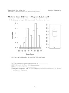
Midterm Exam 1 Review — Chapters 1, 2, 4 and 5
www.stat.ucla.eduStats 11 (Fall 2004) Lecture Note Instructor: Hongquan Xu Introduction to Statistical Methods for Business and Economics Midterm Exam 1 Review — Chapters 1, 2, 4 …
Estimation of Space–Time Branching Process Models in ...
www.stat.ucla.eduEstimation of Space–Time Branching Process Models in Seismology Using an EM–Type Algorithm Alejandro VEEN and Frederic P. SCHOENBERG Maximum likelihood estimation of branching point process models via numerical optimization procedures can be unstable and computa-tionally intensive. We explore an alternative estimation method based on the ...
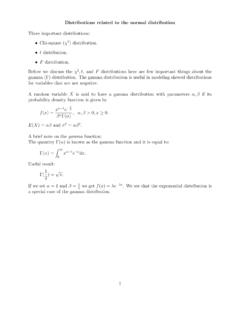
Distributions related to the normal distribution - Website
www.stat.ucla.eduDistributions related to the normal distribution Three important distributions: Chi-square (˜2) distribution. tdistribution. Fdistribution. Before we discuss the ˜2;t, and F distributions here are few important things about the gamma distribution.
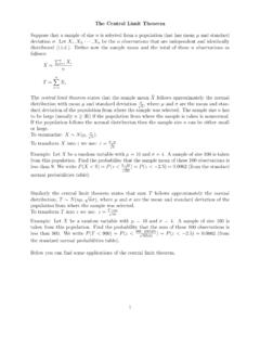
The Central Limit Theorem - Main Concepts
www.stat.ucla.eduCentral limit theorem - proof For the proof below we will use the following theorem. Theorem: Let X nbe a random variable with moment generating function M Xn (t) and Xbe a random variable with moment generating function M X(t). If lim n!1 M Xn (t) = M X(t) then the distribution function (cdf) of X nconverges to the distribution function of Xas ...
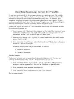
Describing Relationships between Two Variables
www.stat.ucla.eduIs the relationship strong (clear patterns) or weak (fuzzy patterns)? Here are some examples: This data comes from class. The picture comes from plotting each person’s height and weight. For example ( 74, 180), (69, 175), (76, 170), etc. This is a positive relation, fairly …

Covariance and correlation - Main Concepts
www.stat.ucla.eduCorrelation: However, the covariance depends on the scale of measurement and so it is not easy to say whether a particular covariance is small or large. The problem is solved by standardize the value of covariance (divide it by ˙ X˙ Y), to get the so called coe cient of correlation ˆ XY. ˆ= cov(X;Y) ˙ X˙ Y; Always, 1 ˆ 1 cov(X;Y) = ˆ ...
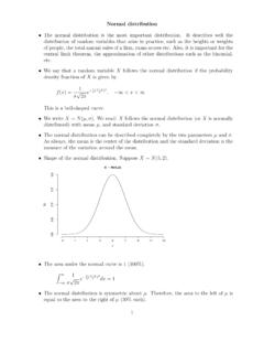
Normal distribution - University of California, Los Angeles
www.stat.ucla.eduWe say that a random variable X follows the normal distribution if the probability density function of Xis given by f(x) = 1 ˙ p 2ˇ e 1 2 (x ˙)2; 1 <x<1 This is a bell-shaped curve. We write X˘N( ;˙). We read: Xfollows the normal distribution (or Xis normally distributed) with mean , and standard deviation ˙.
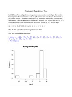
Bootstrap Hypothesis Test - University of California, Los ...
www.stat.ucla.eduWhat if we used the t-test? Since the data now look normal, there’s no reason not to. > t.test(betterspeed,alternative="two.sided",mu=33.02) One Sample t-test data: betterspeed t = -4.6078, df = 17, p-value = 0.0002508 alternative hypothesis: true mean is not equal to 33.02 95 percent confidence interval: 23.83863 29.60582 sample estimates ...
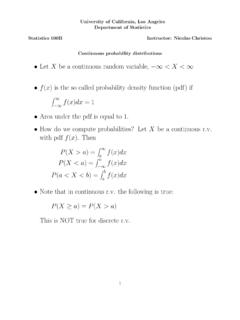
Z f x dx = 1 be a continuous r.v. f x
www.stat.ucla.eduSuppose Xfollows the exponential distribution with = 1. If Y = p X nd the pdf of Y. Example 2 Let X ˘N(0;1). If Y = eX nd the pdf of Y. Note: Y it is said to have a log-normal distribution. Example 3 Let Xbe a continuous random variable with pdf f(x) = 2(1 x);0 x 1. If Y = 2X 1 nd the pdf of Y. Example 4 Let Xbe a continuous random variable ...
Related documents
University of Toronto
www.utstat.toronto.eduProbability and Statistics The Science of Uncertainty Second Edition Michael J. Evans and Je⁄rey S. Rosenthal University of Toronto