1 Finite Element Analysis Methods - Rice University

1 Draft Copyright 2009. All rights reserved. 7 1 finite element analysis methods Introduction The Finite Element method (FEM) rapidly grew as the most useful numerical Analysis tool for engineers and applied mathematicians because of it natural benefits over prior approaches. The main advantages are that it can be applied to arbitrary shapes in any number of dimensions. The shape can be made of any number of materials. The material properties can be non homogeneous (depend on location) and/or anisotropic (depend on direction). The way that the shape is supported (also called fixtures or restraints) can be quite general, as can the applied sources (forces, pressures, heat flux, etc.). The FEM provides a standard process for converting governing energy principles or governing differential equations in to a system of matrix equations to be solved for an approximate solution. For linear problems such solutions can be very accurate and quickly obtained.

2 Having obtained an approximate solution, the FEM provides additional standard procedures for follow up calculations (post processing), such as determining the integral of the solution, or its derivatives at various points in the shape. The post processing also yields impressive color displays, or graphs, of the solution and its related information. Today, a second post processing of the recovered derivatives can yield error estimates that show where the study needs improvement. Indeed, adaptive procedures allow automatic corrections and re solutions to reach a user specified level of accuracy. However, very accurate and pretty solutions of models that are based on errors or incorrect assumptions are still wrong. When the FEM is applied to a specific field of Analysis (like stress Analysis , thermal Analysis , or vibration Analysis ) it is often referred to as Finite Element Analysis (FEA). FEA is the most common tool for stress and structural Analysis .

3 Various fields of study are often related. For example, distributions of non uniform temperatures induce non obvious loading conditions on solid structural members. Thus, it is common to conduct a thermal FEA to obtain temperature results that in turn become input data for a stress FEA. FEA can also receive input data from other tools like motion (kinetics) Analysis systems and computation fluid dynamic (CFD) systems. Basic Integral Formulations The basic concept behind the FEM is to replace any complex shape with the union (or summation) of a large number of very simple shapes (like triangles) that are combined to correctly model the original part. The smaller simpler shapes are called Finite elements because each one occupies a small but Finite sub domain of the original part. They contrast to the infinitesimally small or differential elements used for centuries to derive differential equations.

4 To give a very simple example of this dividing and summing process, consider calculating the area of the arbitrary shape shown in Figure 1 1 (left). If you knew the equations of the bounding curves you, in theory, could integrate them to obtain the enclosed area. Alternatively, you could split the area into an enclosed set of triangles (cover the shape with a mesh) and sum the areas of the individual triangles: . Now, you have some choices for the type of triangles. You could pick straight sided (linear) triangles, or quadratic triangles (with edges that are parabolas), or cubic triangles, etc. The area of a straight sided triangle is a simple algebraic expression. The area of a curved triangle is relatively easy to calculate by numerical integration, but is computationally more expensive to obtain than that for the linear triangle. The first two triangle mesh choices are shown in Figure 1 1 for a large Element size.

5 Clearly, the simple straight sided triangular mesh (on the left) approximates the area very closely, but at the same time introduces geometric errors along the boundary. The boundary geometric error in a linear triangle mesh results from replacing a FEA Concepts: SW Simulation Overview Akin Draft Copyright 2009. All rights reserved. 8 boundary curve by a series of straight line segments. That geometric boundary error can be reduced to any desired level by increasing the number of linear triangles. But that decision increases the number of calculations and makes you trade off geometric accuracy versus the total number of required area calculations and summations. Area is a scalar, so it makes sense to be able to simply sum its parts to determine the total value, as shown above. Other topics, like kinetic energy or strain energy, can be summed in the same fashion.

6 Indeed, the very first applications of FEA to structures was based on minimizing the energy stored is a linear elastic material. The FEM always involves some type of governing integral statement. That integration is also converted to the sum of the integrals over each Element in the mesh. Even if you start with a governing differential equation, it gets converted to an equivalent integral formulation by one of the Methods of weighted residuals (MWR). The two most common Methods , for FEA, are the Galerkin Method and the Method of Least Squares Figure. Figure 1 1 An area crudely meshed with linear and quadratic triangles You may think that the geometric boundary error cited for the linear triangles is eliminated by choosing to use the mesh of curved quadratic triangles (on the right). The parabola segments pass through three points lying exactly on the boundary curve, but can degenerate to straight lines in the interior.

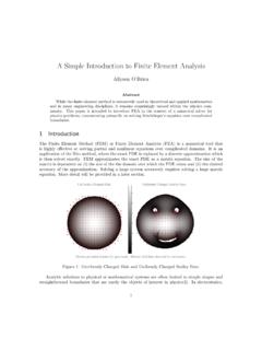
7 (To speed plotting of small elements , most systems draw all the parabolas as two straight line segments, as on the right in Figure 1 1.) Thus, the boundary shape error is indeed reduced, at the expense of more complicated area calculations, but it is not eliminated. Some geometric error remains because most engineering curves are circular arcs, splines, or nurbs (non uniform rational B splines) and thus are not matched by a parabola. The most common way to reduce mesh geometric error is to simply use smaller elements , like Figure 1 2 shows. The default Element choice in SW Simulation is the quadratic Element . Other systems offer a wider range of edge polynomial degree ( cubic), as well as other shapes like quadrilaterals or rectangles. In three dimensional solid applications some systems offer dozens of choices for the edge degree polynomial order, and shapes including hexahedral, wedges, and tetrahedral elements .

8 Hexahedral elements are generally more accurate, but can be more challenging to mesh automatically. Tetrahedral elements can match hexahedral Element performance by using more (smaller) elements , and tetrahedral elements are much easier to mesh automatically. SW Simulation uses only tetrahedral elements for solid studies. An example of the small two dimensional geometric boundary error due to different curved shapes is seen in Figure 1 3 where a circular arc and a parabola pass through the same three points. (A new method, called isogeometric Analysis , can essentially eliminate all geometric errors, but it introduces new approximations in other study stages, such as in the restraint conditions.) FEA Concepts: SW Simulation Overview Akin Draft Copyright 2009. All rights reserved. 9 Figure 1 2 Mesh refinement quickly reduces geometric boundary errors for linear (left) or quadratic elements Figure 1 3 Linear or parabolic elements never exactly match circular shapes Stages of Analysis and Their Uncertainties A FEA always involves a number of uncertainties that impact the accuracy or reliability of each stage of a FEA and its results.

9 The book, Building Better Products with Finite Element Analysis by Adams and Askenazi [1] gives an outstanding detailed description of most of the real world uncertainties associated with solid mechanics FEA. All engineers conducting stress studies should read it. That book also points out how poor solid modeling skills can adversely affect the ability to construct meshes for any type of FEA. Here, the most important FEA uncertainties are highlighted. The typical stages of a FEA study are listed below: 1. Construct the part(s) in a solid modeler. It is surprisingly easy to accidentally build flawed models with tiny lines, tiny surfaces or tiny interior voids. The part will look fine, except with extreme zooms, but it may fail to mesh. Most systems have checking routines that can find and repair such problems before you move on to a FEA study. Sometimes you may have to export a part, and then import it back with a new name because imported parts are usually subjected to more time consuming checks than native parts.

10 When multiple parts form an assembly, always mesh and study the individual parts before studying the assembly. Try to plan ahead and introduce split lines into the part to aid in mating FEA Concepts: SW Simulation Overview Akin Draft Copyright 2009. All rights reserved. 10 assemblies and to locate load regions and restraint (or fixture or support) regions. Today, construction of a part is probably the most reliable stage of any study. 2. Defeature the solid part model for meshing. The solid part may contain features, like a raised logo, that are not necessary to manufacture the part, or required for an accurate Analysis study. They can be omitted from the solid used in the Analysis study. That is a relative easy operation supported by most solid modelers (such as the suppress option in SW) to help make smaller and faster meshes. However, it has the potential for introducing serious, if not fatal, errors in a following engineering study.