Transcription of 1 Properties and Inverse of Fourier Transform
1 Indian Institute of Technology BombayDept of Electrical EngineeringHandout 9EE 603 Digital Signal Processing and ApplicationsLecture Notes 3 August 28, 20161 Properties and Inverse of Fourier TransformSo far we have seen that time domain signals can be transformed to frequency domain bythe so called Fourier Transform . We will introduce a convenient shorthand notationx(t)FT X(f),to say that the signalx(t)has Fourier TransformX(f). Observe that the Transform isnothing but a mathematical operation, and it does not care whether the underlying variablestands for time, frequency, space or something else. Clearly it should remain true thatx(f)FT X(t).This suggests that there should be a way to invert the Fourier Transform , that we cancome back fromX(f)tox(t). If the correspondence fromx(t)toX(f)is a bijection,then we can uniquely invertX(f).
2 This is true for a wide class of functions, in particular,for those class of signals where both the signal and its Fourier Transform are can be extended to cover most signals that we deal with in this class. So we assumesome regularity Properties for the discussion here, that all the integrals are well defined etc,without explicitly stating these each time. Let us first list some Properties of the FourierTransform. Assume thatx(t)FT X(f) (t )FT exp( j2 f )X(f). (t)exp(j2 f0t)FT X(f f0). (t)FT X ( f)andx ( t)FT X (f). (at)=1 SaSX(fa), a (t)=j2 fX(f)iff(t) 0 withStS .Let us prove the last statement, others are (t)exp( j2 ft)dt=( j2 ft)x(t)S+ +j2 fSexp( j2 ft)x(t)dt=j2 fSx(t)exp( j2 ft)dt=j2 fX(f).In the study of Fourier Transforms, one function which takes a niche position is the Gaussianfunction. This is given byg (t)=1 exp( t2 ),where >0 is a parameter of the function.
3 When =1, we will denote the function asg(t). Let us state a well known (t)dt= can be proved as follows. Sg (t)dt 2=Sg(u)duSg(v)dv=1 SSexp( (u2+v2) )dudv=1 S 0S2 0exp( r2 )rd dr=2 Sexp( r2 )rdr= S 0exp( t )dt= Step 3 above, we converted to polar coordinates for solving the integral. The pivotalrole of Gaussian functions follows from the fact that the Fourier Transform of a Gaussianfunction is another Gaussian function. In particular,exp( t2)FT exp( f2) (t)FT g(f)when = the above , applying the scaling property, we also haveg(t)FT g( f)=exp( j f2), > cute aspect of the above formula is that both sides are Gaussians. Thus the formulafrom left to right can be traced in the reverse manner. In other words, we have obtainedthe Fourier inversion formula for Gaussian functions, essentially for free. More specifically,the inversion formula isg (t)=SG (f)exp(j2 ft)df,whereG (f) =exp( f2).
4 Can we extend this to other functions? This is possible if wemake a seemingly simple, but appealing, observation. What happens tog (t)when can takelim 0g (t)= (t).Clearly, all the required Properties of Dirac delta are satisfied by the LHS. In particularlim 0g (t) x(t)=x(t),(1)for all points of continuity for any integrable functionx(t)(proof done in class).tfGalpha(f)FT Figure 1: Illustratingg (t)andG (f)as about the Fourier Transform ofg (t)as 0. It is evident thatG (f)=exp( f2)will end up approximating a constant function in any bounded interval, as 0 (see Figure 1). We know that for integrable functionslimT SStS TSx(t)Sdt= while dealing with the class of integrable functions, we can takelim 0g (t)FT lim 0G (f).The informality in the above equation is that we only know the Fourier Inverse formula whenthere are no limits on both sides.
5 Nevertheless, we make a symbolic representation whichwill make life so much easier that all other jargon/maths so far can be nearly dispensedwith. From now onward, we take the following as a fact, and feel free to apply this withoutmuch ado (If interested there are several treatments on the theory of distributions whichwill give a rigorous justification). (t)FT 1{f R}.(2)Notice that the right side is nothing but a constant function of unit amplitude. What iseven more remarkable is that the formalism in (2) can also be applied while dealing withseveral classes of non-integrable signals. In fact, for all the engineering applications in thiscourse, (2) will be treated as a theorem, or Fourier InverseIt turns out that (2) is all that we need to find the Fourier Inverse , whenever both thefunction and its Transform are integrable. However, we have defined a Dirac delta in anoperational manner, and for (2) to be true, both the function as well as its Fourier transformshould decay sufficiently fast when the respective arguments to these functions are largeenough in magnitude.
6 For the time being, let us throw caution to the wind, and Formulax(t)=SX(f)exp(j2 ft)df.(3)To prove this using (2), let us writeSX(f)exp(j2 ft)df=SSx( )exp( j2 f )d exp(j2 ft)df=Sx( )Sexp( j2 f(t ))dfd =Sx( ) (t )d =x(t).The real power of this theorem from an engineering standpoint is perhaps not in having anintegral formula, but in realizing that we can simply identify the Fourier Inverse ofX(f)asthat functionx(t)which gives the required Fourier Transform . Thus, we can identify thatsinc(f )has Fourier inverse1 rect (t). More generally, we chose notationx(t)FT X(f)toclearly indicate that you can go in both directions, the RHS is the Fourier Transformof the LHS, and conversely, the LHS is the Fourier Inverse of the Transform or SeriesWe have made some progress in advancing the two concepts of Fourier Series and FourierTransform.
7 Which of them to use, we do not have such a freedom as of now. Some studentswere confused about this aspect, with the following comment. Sometimes the teacher uses the Fourier series representation, and some other times theFourier Transform Our lack of freedom has more to do with our mind-set. Fourier Series representationis for periodic signals while Fourier Transform is for aperiodic (or non-periodic) an integrable signal which is non-zero and bounded in a known interval[ T2,T2],and zero elsewhere. This signal will have a Fourier Transform . Will it have a FourierSeries? Yes!, but with the underlying imagination that we have to repeat the signal intime by some interval greater than or equal toT, to make it a periodic one. AT periodicrepetition has the effect ofremovingall frequency components from the Fourier Transformother than those which are multiples of1T.
8 This is consistent with our interpretation of theFourier section is aimed at providing a unified view to Fourier Series and Fourier will argue that everything can be viewed as Fourier Transform , in a generalized key tool-kit which can be of great use is called the Dirac Formalisms, which definessymbolic/formal rules by which we can seamlessly move from Fourier Transform to formalisms allow the identification of Fourier Series as nothing but scaled samples ofthe Fourier Transform . This result can also be alluded to a well known formula calledPoisson s sum the way, picking certain components from a continuous signal is calledsampling, avery important tool for signal processing. Sampling and corresponding signal reconstructionallow us to move between continuous valued signals and discrete ones in a seamless fashion,which is often necessary in today s digital/discrete world.
9 By using Dirac formalisms, itwill become evident that the laws governing sampling are same as the ones that connectFourier Series and SamplingSampling literally means picking up the values from a fewplaces. In discrete countablesituations it means choosing a few objects out of the available ones. Unfortunately thesituation is not that simple when it comes to sampling a continuous time signal to get adiscrete-time one. Let us go through an (x)= 2: Sampling a sine waveIn Figure 2, it is evident that sampling at4 samples per second will yield pictorially thepoints represented by the black dots. These values are convenient to store and they present a difficulty when we wish to convert them back to a continuous timesignal. Why?. To understand this, imagine a continuous time filter (LTI system) whichtakes the samples as input and outputs some waveform ( for example, an interpolator incontinuous time.)
10 H( )Output identi-cally zero!The convolution integral will not recognize the discrete samples as h( )x(t )d =0.(4)We need a formalism to side-step such difficulties. We were in a similar situation a whileback, when we introduced the Dirac formalism to define an impulse, so that the convolutionof any continuous time signal with a Dirac is well defined. We can extend that formalismto sampling too. Instead of samples, we will be dealing with sample and hold. , thesampled value represents an impulse with area equal to the value of the function at thatpoint. With this additional formalism, we can seamlessly move between continuous anddiscrete time in almost all physical situations and engineering this new formalism for samples, Figure 3 shows the output when the waveformsin(x)sampled at intervals of 4are fed into a linear 40 4 h( )The output is something that we expect and logical.