Transcription of 11. Hypersonic Aerodynamics - Virginia Tech
1 7/31/16 11-1 Space Shuttle in NASA Langley Helium Tunnel at M = 20 (NASA SP-440) 11. Hypersonic Aerodynamics Introduction Hypersonic vehicles are commonplace. There are many more of them than the supersonic aircraft discussed in the last chapter. Applications include missiles, launch vehicles and entry bodies. A huge effort has been made developing Hypersonic Aerodynamics methods and configurations. This began with missiles, including the intercontinental ballistic missile (ICBM) effort of the 1950s, followed by development work for the Mercury, Gemini and Apollo manned space flight programs. The next major effort was devoted to the Space Shuttle. Work on hypersonics for future entry vehicles and landing of vehicles on other planets continues. Finally, there is a perennial effort to develop atmospheric Hypersonic vehicles.
2 These efforts have resulted in a massive literature, and we will provide references for further study. In this chapter we limit our discussion to the key things to know from a configuration Aerodynamics viewpoint. Despite the effort to develop Hypersonic configurations, there is no exact definition defining the start of the Hypersonic flow regime. Possibilities include: a) Mach numbers at which supersonic linear theory fails b) Where is no longer constant, and we must consider temperature effects on fluid properties. c) Mach numbers from 3 - 5, where Mach 3 might be required for blunt bodies causing large disturbances to the flow, and Mach 5 might be the starting point for more highly streamlined bodies. In this section we will provide a brief outline of the key distinguishing concepts.
3 The books by Bertin and Cummings1 and Anderson2 provide a starting point for further study. Essentially there are five key points to be made: 1. In many cases surface pressure can be estimated fairly easily 2. Control and stability issues lead to different shapes 3. Temperature and aerodynamic heating become critically important 4, Blunt shapes are commonplace 5. Engine-airframe integration is critical 11-2 Configuration Aerodynamics 7/31/16 Our discussion will conclude with a summary of the flight vehicles that have been studied extensively and sometimes even flown. Our interest is in the lessons learned from these configurations. The X-15, shown in Figure 11-1, is the only true manned Hypersonic airplane flown to date. It was rocket powered, and started flight by being dropped from a B-52, so it was purely a research airplane.
4 The first flight was by Scott Crossfield in June of 1959. The X-15 reached 314,750 feet in July of 1962 piloted by Joe Walker. An improved version reached a Mach number of at an altitude of 102,100 feet in October of 1967 with Pete Knight at the controls. The X-15 program flew 199 flights, with the last one being in October of 1968. Milt Thompson s book3 describes the X-15 program, including the crackling sounds the airframe made as it heated up! Figure 11-1. The X-15 (NASA photo) Surface pressure estimation In many cases surface pressures are relatively easy to estimate at Hypersonic speeds. At supersonic speed we have a local relation for two-dimensional flows relating surface slope and pressure, where is the surface inclination relative to the freestream: (11-1) However, this relation is not particularly useful for most cases in actual aircraft configurations.
5 In comparison, Hypersonic rules are useful. The most famous relation is based on the concepts of Newton. Although Newton was wrong for low-speed flow, his idea does apply at Hypersonic speeds. The idea is that the oncoming flow can be thought of as a stream of particles, that lose all their momentum normal to a surface when they hit the surface. This leads to the relation: Mason Hypersonic Aerodynamics 11-3 7/31/16 (11- 2) where is the angle between the flow vector and the surface. Thus you only need to know the geometry of the body locally to estimate the local surface pressure. Also, particles impact only the portion of the body facing the flow, as shown in Figure 11-2. The rest of the body is in a shadow , and the Cp is assumed to be zero.
6 * See Bertin and Cummings1 or Anderson2 for the derivation of this and other pressure-slope rules. Figure 11-2. Shadow sketch, showing region where Cp is zero Two key observations come from the Newtonian pressure rule. First, the Mach number does not appear! Second, the pressure is related to the square of the inclination angle and not linearly as it is in the supersonic formula. This illustrates how the situation in Hypersonic flow is significantly different than the linear flow models at lower speeds. The Newtonian flow model can be refined to improve agreement with data. This form is known as the Modified Newtonian flow formula, (11-3) where the stagnation Cpmax is a function of Mach and , (11-4) and P02 is the stagnation or total pressure behind a normal shock. This expression gets both the Mach number and ratio of specific heats back into the problem.
7 The classical Newtonian theory is actually the limit as M , and 1. These formulas are only valid when is positive. There are lots of other local rules, and Anderson s book2 should be consulted for a more complete discussion. These are known as surface inclination rules. The methods normally heard in Hypersonic discussions include the tangent cone, tangent wedge and shock expansion methods. There is also a modification to the Newtonian pressure rule to include surface curvature effects. This is known as the Newtonian-Busemann rule. How well do these methods work? We look at two cases. First we look at a blunt body case, and then we will compare results with the pressure on a circular cone at zero angle of attack. Figure 11-3 shows the agreement with wind tunnel data for a blunted In this case the agreement is remarkably good for a Mach number of Note also that for many Hypersonic cases we plot with a different axis direction than classic sub- super-sonic Aerodynamics (Note the * Recall Cpvac = -2/( M2), and quickly approaches zero as the Mach number increases.)
8 ShadowRegion,Cp= Configuration Aerodynamics 7/31/16 change in slope at about s/r of The geometry is not a pure hemisphere cone, but has a transition arc). If we had used the pure Newtonian formula the pressure at the nose would have been Clearly the modified formula does an excellent job. Figure 11-3. Comparison of the modified Newtonian estimate over the nose of a blunted cone with wind tunnel data (Model 2 in TN D-4865).4 Next we will examine the results of Newtonian and Modified Newtonian theory together with predictions from a theory given by DeJarnette, et al5 and the exact results from the NASA Cone Figure 11-4 shows the surface pressure results over a Mach number range from 4 to 10, and cone angles of 15 and 25 degrees. The cone table results can be considered to be the exact inviscid values.
9 Recall that the cone produces a conical flowfield, and the surface pressure variation is constant along the surface for an attached shock. In this case the Newtonian approximations are not nearly as good. , surface arc length from stagnation pointM = data,NASA TN D-4865 Modified Newtonian FlowPressure Mason Hypersonic Aerodynamics 11-5 7/31/16 Figure 11-4. Comparison of surface pressures for a cone at zero angle of attack. Since the Newtonian estimates are not particularly good, we will provide the simple formula from DeJarnette5 et al that we ve shown works well: (11-5) where: The advantage of the so-called surface inclination rules is that they only need the local geometry. These methods were combined into a program know as the Hypersonic Arbitrary Body Program (HABP) originally developed at Douglas Aircraft and also known as the Gentry Code.
10 The program is available for free download from the Carmichael s Public Domain Aeronautical Software Unfortunately, the user has to be wise enough to choose which rule should be used over various parts of the body. Once you proceed beyond the early stages of configuration design it is appropriate to use CFD. While we are looking at surface pressures we should look at the change in physics from subsonic to Hypersonic flow. This will be a key concept in configuration development. What is the maximum (fictitious) lift on a flat plate? I call this the ultimate lift. The resulting value is given in Figure 11-5. Here the lower surface pressure is taken equal to the stagnation value and the upper surface pressure is taken equal to the vacuum value.