Transcription of CHAPTER 1 INTRODUCTION TO NUMERICAL METHOD
1 CHAPTER 1 INTRODUCTION TO NUMERICAL METHOD Presenter: Dr. Zalilah Sharer 2018 School of Chemical and Energy Engineering Universiti Teknologi Malaysia 16 September 2018 Chemical Engineering, Computer & NUMERICAL methods Role of Chemical Engineers Chemical engineering covers basic skill in mathematics, chemistry, physic and biology, also engineering practical aspect. Its definition was purposely general because chemical engineers can work in many types of industry. Chemical engineers involve in chemical process that transform raw material into product. It covers all aspect of design, testing, scale-up, operation, control and optimizations. These processes involve solution to huge system of algebraic equation, nonlinear and complex equation, which are difficult to be solved analytically.
2 CHAPTER 2: Approximation and Errors CHAPTER 3: Roots of equations - a variable or parameter that satisfies a single nonlinear equation CHAPTER 4: Linear algebraic equations - a set of values that satisfies a set of linear algebraic equations CHAPTER 5: Curve Fitting - to fit curves to data points CHAPTER 6: NUMERICAL differentiation and integration - - area under a curve CHAPTER 7: Ordinary differential equations - many engineering applications used rate of change Approximations and round-off errors Bracketing methods Linear algebraic equations Least-Squares Regression Newton-cotes integration of equations Runge-Kutta methods Taylor series Open methods Gauss Elimination Interpolation NUMERICAL differentiation Engineering Applications Engineering applications LU decomposition & matrix inversion Engineering Applications Engineering Applications Gauss Seidel and Engineering Applications 3 NUMERICAL methods Roots of equation Linear algebraic Differentiation & Integration Curve fitting Ordinary differential equations NUMERICAL methods Techniques by which mathematical problems are formulated so that they can be solved with arithmetic operations involve large numbers
3 Of calculation NUMERICAL methods Example: Integration Analytical solution: Computer as usual as in calculus NUMERICAL METHOD : Use trapezoidal rule or Simpson s rules Advantages problem-solving tools capable of handling large systems of equations, nonlinearities and complicated geometries that are often impossible to solve analytically to design and develop own programs without having to buy or commission expensive software to reduce higher mathematics to basic arithmetic operations Computers and Software MATLAB, Mathematica, Dynafit etc are some software packages to implement NUMERICAL methods . Help to solve engineering problem in NUMERICAL methods . Else. MS-EXCEL also can be used to solve NUMERICAL problems. Problem Solving Process Problem Solving Process Mathematical model Equations that expresses the essential features of a physical systems Represented as a functional relationship in the form of Dependent Variables = f (independent, parameters, forcing function, variables ) Dependent Variables - Reflects the behavior or state of the system Independent Variables - Dimensions, such as time and space Parameters - Reflective of the system s properties or composition Forcing Function - External influence acting upon it States that the time rate change of momentum of a body is equal to the resulting force acting on it.
4 The model is formulated as F = ma (eqn ) F=net force acting on the body (N) m=mass of the object (kg) a=its acceleration (m/s2) Newton s 2nd law of Motion Equation can be written as: a = F / m eqn simple algebraic equation that can be solved analytically Newton s 2nd law of Motion To determine the terminal velocity of a free-falling body near the earth s surface using Newton 2nd law. Express acceleration as the time rate of change of the velocity (dv/dt) and substituting into eq. ( ) to yield d /dt = F/m (eqn. ) or F = m (d /dt) F +ve : accelerate F -ve : decelerate F = 0 (constant velocity) Express the net force in term of measurable variables and parameters, in which the net force is composed of 2 opposing forces: The downward pull of gravity FD and the upward force of air resistance Fu: F = FD + Fu (eqn.)
5 If downward force is +ve , 2nd law can be used to formulate the force due to gravity, as FD = mg (eqn. ) g = m/s2 The air resistance that acts in an upward direction; Fu = -c (eqn. ) c = drag coefficient (kg/s) Fu FD The net force is the difference between the downward (FD) and upward (FU). By combining eqs. ( ) through ( ) to yield: d /dt = (mg c )/m (eqn. ) or simplifying the right side, d /dt = g (c/m)v (eqn. ) Eq. ( ) is a differential equation. The exact solution of eq. ( ) cannot obtained by simple algebraic manipulation, which needs calculus to obtain an exact or analytical solution. If = 0 at t=0, calculus can be used to solve eq. ( ) for (t)= (gm/c)[1-e-(c/m)t] (eqn. ) This is a differential equation and is written in terms of the differential rate of change dv/dt of the variable that we are interested in predicting.
6 If the parachutist is initially at rest (v=0 at t=0), using calculus tmcecgmtv)/(1)( Independent variable Dependent variable Parameters Forcing function Eq. is called analytical/exact solution because it exactly satisfies the original differential equation. (t) = dependent variable t = independent variable c & m = parameters g = the forcing function However, many mathematical models cannot be solved as shown in eqn. The only alternative is to develop a NUMERICAL solution that approximates the exact solution NUMERICAL METHOD . Mainly from second law of thermodynamics ==> F = ma The model then can be derived with The force acting on the body : F = FU + FD Force on a falling parachute Analytical Solution to the Falling Parachutist Problem A parachutist of mass kg jumps out of a stationary hot air balloon.
7 Use equation to compute velocity for every 2 seconds. The drag coefficient is equal to kg/s and g = m/s2 Example 1 Solution Inserting the parameter into eq. ( ) yields which can be used to compute terminal velocity. v(t) gmc1 e cm t v(t) ( )( ) e t v(t) e Solution Terminal velocity, ut The terminal velocity of a falling body occurs during free fall when a falling body experiences zero acceleration. Using NUMERICAL METHOD Approach The time rate of change of velocity can be approximated using: eqn. 11()( )iiiiv tvdvvdttttt Substituted into eq. ( ) to give: Eq. is called a finite divided difference approximation of the derivative time ti.
8 This eq. then be rearranged to yield: eqn. The term in [brackets] is the differential equation in eq.( ). This provides a means to compute the rate of change or slope of . Eq. can be used to determine the velocity at ti+1(new value of velocity) using slope and initial value for velocity at sometime ti. New value = old value +(slope x step size) 11()( )iiiiiv tvcgvmtttt 11()( )-( )-iiiiicvvgvmtttt t Example 2 Perform the same computation as in Example 1 but use Equation to compute the velocity. Employ a step size of 2 s for the calculation 11()( )-( )-iiiiicvvgvmtttt t Eqn. Solution At start of the computation (ti=0), the velocity of the parachutist is zero. First interval (from t=0 to 2s) For next interval, use t = 2 to 4s The calculation is continued in a similar fashion to obtain additional value 2 2 Solution t,s v,m/s 0 2 4 6 8 10 12 010203040506002468101214t,sv, m/sExact, analytical solution Approximate, NUMERICAL solution Terminal velocity Analytical vs NUMERICAL solution Equation is called analytical or exact solution exactly satisfies the original differential equation (no error) Unfortunately, many mathematical models cannot be solved exactly NUMERICAL methods approximate the exact solution Equation can be used to determine the velocity at time ti+1 if an initial value for velocity at time ti is given.
9 This new value of velocity at ti+1 can in turn be employed to extend the computation to velocity at ti+2 and so on. In general: New value = old value + (slope x step size) This approach is formally called Euler s METHOD Question? THE END Thank You for the Attention