Transcription of Chapter 2: Simple Linear Regression
1 Chapter 2: Simple Linear Regression1 The modelThesimple Linear regressionmodel fornobser-vations can be written asyi= 0+ 1xi+ei, i= 1,2, ,n.(1)The designationsimpleindicates that there is onlyone predictor variablex, andlinearmeans thatthe model is Linear in 0and 1. The intercept 0and the slope 1are unknown constants, andthey are both calledregression coefficients;ei sare random errors. For model (1), we have thefollowing (ei) = 0fori= 1,2, ,n, or, equiva-lentlyE(yi) = 0+ var(ei) = 2fori= 1,2, ,n, or, equiva-lently, var(yi)) = (ei,ej) = 0for alli6=j, or, equivalently,cov(yi,yj) = Ordinary Least Square EstimationThemethod of least squaresis to estimate 0and 1so that the sum of the squares of the differ-ence between the observationsyiand the straightline is a minimum, , minimizeS( 0, 1) =n i=1(yi 0 1xi) = XE(Y|X=x) 1=Slope 0=Intercept1 Figure 1: Equation of a straight lineE(Y|X=x) = 0+ least-squares estimators of 0and 1, say 0and 1, must satisfy 2n i=1(yi 0 1xi) = 0(2) 2n i=1(yi 0 1xi)xi= 0(3)Simplifying these two equations yieldsn 0+ 1n i=1xi=n i=1yi 0n i=1xi+ 1n i=1x2i=n i=1yixi(4)Equations (4) are called theleast-squares nor-mal equations.
2 The solution to the normal equa-tions is 1= ni=1xiyi n x y ni=1x2i n x2= ni=1(xi x)(yi y) ni=1(xi x)2=SxySxx, 0= y 1 difference between the observed valueyiand the corresponding fitted value yiis aresidual, , ei=yi yi=yi ( 0+ 1xi), i= 1,2, ,nUsing Forbe s data, we have x= , y= , Sxy= ,Syy= , the parameter estimates are 1=SxySxx= , 0= y 1 x= estimate line, given by either of the equations E(Lpress|temp) = + fit of this line to the data is excellent as shownin Figure (Pressure) 2: Regression for log(pressure) versus Properties of the least-squares estimators and the fit-ted Regression modelIf the three assumptions in section 1 hold, thenthe least squares estimators 0and 1are unbi-ased and have minimum variance among all linearunbiased estimates (best Linear unbiased estima-tors). (The corresponding Gauss-Markov theoremis proved in Appendix).E( 1) = 1,E( 0) = 0,var( 1) = 2 Sxxvar( 0) = 2(1n+ x2 Sxx)There are several other useful properties of theleast squares fit:1.
3 The sum of the residuals in any regressionmodel that contains an intercept 0is alwayszero, that is,n i=1(yi yi) =n i=1 ei= The sum of the observed valuesyiequals thesum of fitted values yi, orn i=1yi=n i=1 The least squares Regression line always passesthrough the centroid (the point ( y, x)) of The sum of the residuals weighted by the cor-responding value of the regressor variable al-ways equals zero, that isn i=1xi ei= The sum of the residuals weighted by the cor-responding fitted value always equals zero, thatis,n i=1 yi ei= 0,or y e= Estimation of 2 The estimate of 2is obtained from the residualsum of squares (SSRes) or sum of squared error(SSE),SSRes=n i=1e2i=n i=1(yi yi) related formulas are Regression sum of squares(SSR) and total sum of squares (SST)SSR=n i=1( yi y)2= 1 Sxy,SST=n i=1(yi y) they satisfy the following equation,SST=SSR+ unbiased estimate of 2is 2=SSResn 2= The models in the centered formSuppose we redefine the regressor variablexiasthe deviation from its own average, sayxi Regression model then becomesyi= 0+ 1(xi x) + 1 x+ i= ( 0+ 1 x) + 1(xi x) + i= 0+ 1(xi x) + iIt is easy to show that 0= y, the estimator ofthe slope is unaffected by the transformation, andCov( 0, 1) = Hypothesis testing on the slope and interceptHypothesis testing and confidence intervals (nextsection) require that we make the additional as-sumption that the model errors iare normally dis-tributed.
4 Thus, the complete assumptions are that i N(0, 2).Suppose that we wish to test the hypothesis thatthe slope equals a constant, say 10. The appro-priate hypotheses areH0: 1= 10H1: 16= 10(5)Sinceei N(0, 2), we haveyi N( 0+ 1xi, 2)and 1 N( , 2/Sxx). Therefor,Z0= 1 10 2/Sxx N(0,1)if the null hypothesisH0: 1= 10is true. If 2were known, we could useZ0to test the hypothe-sis (5).If 2is unknown, we know that (1)MSResis anunbiased estimator of 2; (2)(n 2)MSRes/ 2follows a 2n 2distribution; and (3)MSResand 1are independent. Therefore,t0= 1 10 MSRes/Sxx= 1 10se( 1)follows atn 2distribution if the null hypothesisH0: 1= 10is true. The null hypothesis is rejected if|t0|> t /2,n testH0: 0= 00H1: 06= 00,(6)we could use the test statistict0= 0 00 MSRes(1n+ x2 Sxx)= 0 00se( 0).A very important special case of the hypothesisin (5) isH0: 1= 0H1: 16= 0,(7)Failing to reject the null hypothesis implies that thereis no Linear relationship the snowfall data, 1= , andse( 1) = Thus,t= ( 0) = Comparingtwith the critical valuet( ,91) = , we conclude that early and late season snow-falls are The analysis of varianceWe may also use an analysis of variance approachto test significance of Regression .
5 The analysis ofvariance is based on the fundamental analysis ofvariance identity for a Regression model, ,SST=SSR+ 1degrees of freedom be-cause one degree of freedom is lost as a result ofconstraint ni=1(yi y)on the deviationsyi y;SSRhasdfR= 1degree of freedom becauseSSRis completely determined by one parameter,namely, 1;SSReshasdfRes=n 2degrees offreedom because two constraints are imposed onthe deviationsyi yias a result of estimating 0and 1. Note that the degrees of freedom have anadditive property:dfT=dfR+dfResn 1 = 1 + (n 2)We can show: (1) thatSSRes/ 2= (n 2)MSRes/ 2follows a 2n 2distribution; (2) thatif the null hypothesisH0: 1= 0is true, thenSSR/ 2follows a 21distribution; and (3) thatSSResandSSRare independent. By the definition of anFstatistic,F0=SSR/dfRSSRes/dfRes=SSR/1 SSRes/(n 2)=MSRMSR esfollows theF1,n 2distribution. IfF0> F ,1,n 2we reject the null hypothesisH0: 1= 0. Therejection region is single-sided, due to that (Ap-pendix )E(MSRes) = 2, E(MSR) = 2+ 21 Sxx,Source of Sum ofDegrees of MeanF0 Variation SquaresFreedom SquareRegressSSR= 1 Sxy1 MSRMSRMSResResidualSSRes=SST 1 Sxyn 2 MSResTotalSSTn 1 Table 1: Analysis of Variance (ANOVA) for testing significance of regressionthat is, it is likely that the slope 16= 0if the ob-served value ofF0is analysis of variance is summarized in thefollowing analysis of variance for Forbes data is givenSource of Sum of Degrees of MeanF0 Variation Squares Freedom SquareRegress 2: Analysis of Variance (ANOVA) for Forbes Table Coefficient of determinationThe quantityR2=SSRSST= 1 SSResSSTis called the coefficient of determination.
6 For Forbes data,R2= ,and thus the variability in the ob-served values is explained by boiling the below, we list some properties The range ofR2is0 R2 1. If all the j swere zero, except for 0,R2would be zero.(This event has probability zero for continuousdata.) If all they-values fell on the fitted sur-face, that is, ifyi= yi,i= 1,2, ,n, thenR2would be Adding a variablexto the model increases(cannot decrease) the value invariant to a scale change not measure the appropriateness ofthe Linear model, forR2will often be largeeven thoughyandxare nonlinearly Interval estimation in Simple Linear Confidence intervals on 0, 1and 2 The width of these confidence intervals is a mea-sure of the overall quality of the Regression the errors are normally and independently dis-tributed, then the sampling distribution of both 1 1se( 1)and 0 0se( 0)istwithn 2degrees of freedom. Therefore,a100(1 )percent confidence interval on theslope 1is given by 1 t /2,n 2se( 1) 1 1+t /2,n 2se( 1)and a100(1 )percent confidence interval onthe intercept 0is 0 t /2,n 2se( 0) 0 0+t /2,n 2se( 0)Frequency interpretation.
7 If we were to take repeatedsamples of the same size at the samplexlevelsand construct, for example,95%confidence inter-vals on the slope for each sample, then95%ofthose intervals will contain the true value of Forbes data,se( 0) = (1/17 +( )2 )1/2= , andse( 1) = / Sxx= For a90%confidence inter-val,t( ,15) = , and the interval is ( ) 0 + ( ) 0 interval for the slope ( ) 1 + ( ) 1 the errors are normally and independently dis-tributed, then the sampling distribution of(n 1)MSRes/ 2is chi-square with(n 2)degrees of ,P{ 21 /2,n 2 (n 2)MSRes 2 2 /2,n 2}= 1 and consequently a100(1 )percent confidenceinterval on 2is(n 2)MSRes 2 /2,n 2 2 (n 2)MSRes 21 /2,n Interval estimation of the mean responseLetx0be the level of the regressor variable forwhich we wish to estimate the mean response, sayE(y|x0). We assume thatx0is any value of theregressor variable within the range of the originaldata onxused to fit the model.
8 An unbiased pointestimator ofE(y|x0)is E(y|x0) = y|x0= 0+ variance of y|x0isV ar( y|x0) =V ar[ y+ 1(x0 x)] = 2[1n+(x0 x)2 Sxx]since cov( y, 1) = 0. Thus, the sampling distribu-tion of y|x0 E(y|x0) MSRes(1/n+ (x0 x)2/Sxx)istwithn 2degrees of freedom. Consequently,a 100(1 )percent confidence interval on themean response at the pointx=x0is y|x0 t /2,n 2 MSRes(1/n+ (x0 x)2/Sxx) E(y|x0) y|x0+t /2,n 2 MSRes(1/n+ (x0 x)2/Sxx)(8)10 Prediction of new observationsAn important application of the Regression modelis prediction of new observationsycorrespondingto a specified level of the regressor variablex. Ifx0is the value of the regressor variable of interest,then y0= 0+ 1x0is the point estimate of the new value of the re-sponsey0. Now consider obtaining an interval es-timate of this future observationy0. The confi-dence interval on the mean response atx=x0is inappropriate for this problem because it is aninterval estimate on the mean ofy(a parameter),not a probability statement about future observa-tions from the =y0 y0is normally distributed withmean 0 and varianceV ar( ) = 2[1 +1n+(x0 x)2 Sxx].
9 Thus, the100(1 )%percent prediction intervalon a future observation atx0is y0 t /2,n 2 MSRes(1 + 1/n+ (x0 x)2/Sxx) y0 y0+t /2,n 2 MSRes(1 + 1/n+ (x0 x)2/Sxx)(9)By comparing (8) and (9), we observe that theprediction interval atx0is always wider than theconfidence interval atx0because the predictioninterval depends on both the error from the fittedmodel and the error associated with future may generalize (9) somewhat to find a100(1 )percent prediction interval on the mean ofmfuture observations on the response atx0. The100(1 )%prediction interval on y0is y0 t /2,n 2 MSRes(1/m+ 1/n+ (x0 x)2/Sxx) y0 y0+t /2,n 2 MSRes(1/m+ 1/n+ (x0 x)2/Sxx).(10)For prediction of100 log(Pressure)for alocation withx0= 200, the point prediction is y0= + (200) = ,with standard error of (1 +117+(200 ) )1/2= , a99%predictive interval ( ) y0 + ( ), y0 a99%predictive interval for Pressure Pressure , Pressure The ResidualsPlots of residuals versus other quantities are usedto find failures of assumptions.
10 The most commonplot, especially useful in Simple Regression , is theplot of residuals versus the fitted values. A null plot indicate no failure of assumptions. Curvature might indicate that the fitted meanfunction is inappropriate. Residuals that seem to increase or decreasein average magnitude with the fitted values mightindicate nonconstant residual variance. A few relatively large residuals may be indica-tive of outliers, case for which the model issomehow plot of residuals versus fitted values for theheights data is shown in Figure 3. This is a fitted values and residuals for Forbes dataare plotted in Figure 4. This plot indicates thatcase 12 is an outlier. Delete this point from thedataset. Refitting the model resulting in the follow-ing results (Table 3):Table 3: Summary statistics for Forbes data with all data and with case 12 All data Delete case 12 ( 0) ( 1) 505 Fitted valuesResidualsFigure 3: Residuals versus fitted values for the heights valuesResiduals12 Figure 4: Residual plot for Forbes data.