Chapter 33

1 Chapter . The z-Transform 33. Just as analog filters are designed using the laplace transform, recursive digital filters are developed with a parallel technique called the z-transform. The overall strategy of these two transforms is the same: probe the impulse response with sinusoids and exponentials to find the system's poles and zeros. The laplace transform deals with differential equations, the s-domain, and the s-plane. Correspondingly, the z-transform deals with difference equations, the z-domain, and the z-plane. However, the two techniques are not a mirror image of each other; the s-plane is arranged in a rectangular coordinate system, while the z-plane uses a polar format. Recursive digital filters are often designed by starting with one of the classic analog filters, such as the Butterworth, Chebyshev, or elliptic. A series of mathematical conversions are then used to obtain the desired digital filter.

2 The z-transform provides the framework for this mathematics. The Chebyshev filter design program presented in Chapter 20 uses this approach, and is discussed in detail in this Chapter . The Nature of the z-Domain To reinforce that the laplace and z-transforms are parallel techniques, we will start with the laplace transform and show how it can be changed into the z- transform. From the last Chapter , the laplace transform is defined by the relationship between the time domain and s-domain signals: 4. m X (s) ' x (t ) e & s t dt t ' &4. where x (t) and X (s) are the time domain and s-domain representation of the signal, respectively. As discussed in the last Chapter , this equation analyzes the time domain signal in terms of sine and cosine waves that have an exponentially changing amplitude. This can be understood by replacing the 605. 606 The Scientist and Engineer's Guide to Digital Signal Processing complex variable, s, with its equivalent expression, F % jT.

3 Using this alternate notation, the laplace transform becomes: 4. m X (F, T) ' x (t ) e & F t e & jTt dt t ' &4. If we are only concerned with real time domain signals (the usual case), the top and bottom halves of the s-plane are mirror images of each other, and the term, e & jTt , reduces to simple cosine and sine waves. This equation identifies each location in the s-plane by the two parameters, F and T . The value at each location is a complex number, consisting of a real part and an imaginary part. To find the real part, the time domain signal is multiplied by a cosine wave with a frequency of T , and an amplitude that changes exponentially according to the decay parameter, F . The value of the real part of X (F,T). is then equal to the integral of the resulting waveform. The value of the imaginary part of X (F,T) is found in a similar way, except using a sine wave. If this doesn't sound very familiar, you need to review the previous Chapter before continuing.

4 The laplace transform can be changed into the z-transform in three steps. The first step is the most obvious: change from continuous to discrete signals. This is done by replacing the time variable, t, with the sample number, n, and changing the integral into a summation: j x [n] e 4. & F n & jTn X (F, T) ' e n ' &4. Notice that X (F,T) uses parentheses, indicating it is continuous, not discrete. Even though we are now dealing with a discrete time domain signal, x[n] , the parameters F and T can still take on a continuous range of values. The second step is to rewrite the exponential term. An exponential signal can be mathematically represented in either of two ways: y [n ] ' e & F n or y [n ] ' r -n As illustrated in Fig. 33-1, both these equations generate an exponential curve. The first expression controls the decay of the signal through the parameter, F . If F is positive, the waveform will decrease in value as the sample number, n, becomes larger.

5 Likewise, the curve will progressively increase if F is negative. If F is exactly zero, the signal will have a constant value of one. Chapter 33- The z-Transform 607. a. Decreasing 3. y [n] ' e & Fn, F ' 2. y[n]. or 1. y [n] ' r-n, r ' 0. -10 -5 0 5 10. n FIGURE 33-1. Exponential signals. Exponentials can be represented in two different b. Constant 3. mathematical forms. The laplace transform uses one way, while the y [n] ' e & Fn, F ' 2. z-transform uses the other. y[n]. or 1. y [n] ' r-n, r ' 0. -10 -5 0 5 10. n c. Increasing 3. y [n] ' e & Fn, F ' & 2. or y[n]. 1. y [n] ' r-n, r ' 0. -10 -5 0 5 10. n The second expression uses the parameter, r, to control the decay of the waveform. The waveform will decrease if r > 1 , and increase if r < 1. The signal will have a constant value when r ' 1 . These two equations are just different ways of expressing the same thing. One method can be swapped for the other by using the relation: r-n ' [ e ln ( r ) ]-n ' e-n ln ( r ) ' e & Fn where: F ' ln ( r ).

6 The second step of converting the laplace transform into the z-transform is completed by using the other exponential form: j x [n ] r e 4. X (r, T) ' -n & j Tn n ' &4. While this is a perfectly correct expression of the z-transform, it is not in the most compact form for complex notation. This problem was overcome 608 The Scientist and Engineer's Guide to Digital Signal Processing in the laplace transform by introducing a new complex variable, s, defined to be: s ' F % jT . In this same way, we will define a new variable for the z- transform: z ' r e jT. This is defining the complex variable, z, as the polar notation combination of the two real variables, r and T. The third step in deriving the z-transform is to replace: r and T , with z. This produces the standard form of the z- transform: j x [n] z EQUATION 33-1 4. &n The z-transform. The z-transform defines X (z) '. the relationship between the time domain n ' &4.

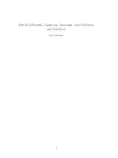
7 Signal, x [n] , and the z-domain signal, X (z) . Why does the z-transform use r n instead of e & Fn , and z instead of s? As described in Chapter 19, recursive filters are implemented by a set of recursion coefficients. To analyze these systems in the z-domain, we must be able to convert these recursion coefficients into the z-domain transfer function, and back again. As we will show shortly, defining the z-transform in this manner ( r n and z) provides the simplest means of moving between these two important representations. In fact, defining the z-domain in this way makes it trivial to move from one representation to the other. Figure 33-2 illustrates the difference between the laplace transform's s-plane, and the z-transform's z-plane. Locations in the s-plane are identified by two parameters: F, the exponential decay variable along the horizontal axis, and T, the frequency variable along the vertical axis.

8 In other words, these two real parameters are arranged in a rectangular coordinate system. This geometry results from defining s, the complex variable representing position in the s- plane, by the relation: s ' F % jT. In comparison, the z-domain uses the variables: r and T, arranged in polar coordinates. The distance from the origin, r, is the value of the exponential decay. The angular distance measured from the positive horizontal axis, T, is the frequency. This geometry results from defining z by: z ' re & jT . In other words, the complex variable representing position in the z-plane is formed by combining the two real parameters in a polar form. These differences result in vertical lines in the s-plane matching circles in the z-plane. For example, the s-plane in Fig. 33-2 shows a pole-zero pattern where all of the poles & zeros lie on vertical lines. The equivalent poles &. zeros in the z-plane lie on circles concentric with the origin.

9 This can be understood by examining the relation presented earlier: F ' & ln(r) . For instance, the s-plane's vertical axis ( , F' 0 ) corresponds to the z-plane's Chapter 33- The z-Transform 609. s - Plane z - Plane Im Im F. r'1. r T. T. Re Re DC DC. (F ' 0, T' 0 ) (r ' 1, T' 0 ). FIGURE 33-2. Relationship between the s-plane and the z-plane. The s-plane is a rectangular coordinate system with F. expressing the distance along the real (horizontal) axis, and T the distance along the imaginary (vertical) axis. In comparison, the z-plane is in polar form, with r being the distance to the origin, and T the angle measured to the positive horizontal axis. Vertical lines in the s-plane, such as illustrated by the example poles and zeros in this figure, correspond to circles in the z-plane. unit circle (that is, r ' 1 ). Vertical lines in the left half of the s-plane correspond to circles inside the z-plane's unit circle.

10 Likewise, vertical lines in the right half of the s-plane match with circles on the outside of the z-plane's unit circle. In other words, the left and right sides of the s-plane correspond to the interior and the exterior of the unit circle, respectively. For instance, a continuous system is unstable when poles occupy the right half of the s-plane. In this same way, a discrete system is unstable when poles are outside the unit circle in the z-plane. When the time domain signal is completely real (the most common case), the upper and lower halves of the z-plane are mirror images of each other, just as with the s- domain. Pay particular attention to how the frequency variable, T , is used in the two transforms. A continuous sinusoid can have any frequency between DC and infinity. This means that the s-plane must allow T to run from negative to positive infinity. In comparison, a discrete sinusoid can only have a frequency between DC and one-half the sampling rate.