Coaxial Cable Delay - VE2AZX

1 Coaxial Cable Delay By: Jacques Audet VE2 AZX. Introduction Last month, I reported the results of measurements on a number of Coaxial cables with the VNA. (Vector Network Analyzer). (Ref. 3) This month, I describe the measurement technique and theory behind these measurements. I will also try to give an insight on what is happening. Transmission lines are described by their two most important characteristics: the characteristic impedance Zo and the Delay . For instance, take a short (say wavelength) piece of Coaxial Cable such RG-58U and measure its capacitance with the other end open.

2 A one foot length yields ~ pF. The inductance may also be measured with the other end shorted. It yields ~ nH. The impedance may now be computed as: L 10 9. Zo = Eq.(1) Zo = = ohms Close enough to 50 ohms. C 10 12. Here L and C are measured for the same length. The Delay may also be computed: Delay = L C Eq. (2) Delay = 10 9 10 12 = nSec For an ideal line, the Delay increases linearly with its length, while its impedance remains constant. Let's compute the velocity in foot per second: len 1. v= Eq. (3) v= 9. = 108 foot per second or *108 meters/second Delay 10. This is less than the speed of light.

3 The ratio of the above speed to the speed of light gives us the velocity factor Vf: 108. Vf = = or % of the speed of light. 108. Keep in mind that these results have been obtained with only two measurements. As mentioned earlier, the Delay increases linearly with the line length. For a given length, the phase difference between the input and output will increase with the frequency: = 2 f Delay Eq. (4) Here the phase is in radians and the frequency f is in Hertz. 360. Converting the phase from radians to degrees requires multiplying by: 2 . At 162 MHz, the phase Delay in degrees will be: deg = f 360 Delay = 162 106 360 10 9 This length that gives 90 degrees of phase shift is also known as a quarter wavelength.

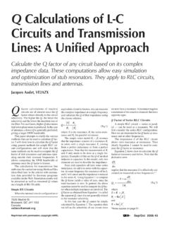
4 Measuring Delay with the Vector Network Analyzer The instrument measures the phase over a frequency range of interest. In the above example, we get ~ 90 degrees of phase shift form 0 Hz to 162 MHz. Therefore the Delay may be computed from the previous equation. Figure 1. An ideal transmission line gives a linear change of phase versus frequency. The slope of these phase curves gives us the Delay : deg Delay = = Eq. (5). 360 f Where is the change in phase in radians, the change in the frequency in radians/sec. Figure 2. The Delay may be computed from the change in phase over a small frequency increment.

5 In practice, the phase behavior of real transmission lines is not perfectly linear. By measuring the delta phase ( ) for a small frequency increment ( ), we get the actual Delay over a small group of frequencies. This actual Delay is called group Delay , as it gives the Delay for a group of frequencies, also called the aperture. We try to use a frequency aperture as small as possible to be able to view all peaks and valleys in the group Delay . This tends to give more noise in the phase measurement as the aperture is reduced. So a compromise aperture must be used that will only give a tolerable amount of noise on the group Delay trace.

6 The VNA measures the phase for a number of frequency points, such as 201 points over a span of frequencies. The frequency aperture is specified as a percentage of the frequency span. Typical aperture values range from 1 % to 10 % of span. Figure 3 shows the phase versus frequency for a real transmission line. Figure 3. Delay Variations Caused by Changes in Inductance What is causing Delay variations ? Equation 2 tells us that the Delay is related to the distributed inductance and capacitance of the line. These appear to be constants related to the line geometry and to the dielectric constant of the insulation.

7 Remember also that the inverse of the Delay (per unit length) is the velocity of propagation. The effective distributed inductance L has two components which may be considered in series: the external inductance Le and the internal inductance Li. The first component Le is the inductance created by the flux outside the conductors, between the inner and the outer conductors. It is the normal inductance that we assume to be constant. The internal inductance Li comes from the flux internal to the conductor. It can only exist if the conductor is not perfect. Even copper or silver is not a perfect conductor and a small part of the flux exists mainly inside the center conductor.

8 This internal flux exists mostly where the current penetrates inside the conductor. That is at the skin depth, which decreases as the frequency increases. For instance copper has a skin depth of mil at 1 MHz, decreasing by a factor of 1/square root(10) at 10 MHz. At 100 MHz, the skin depth is mil. The shin depth increases for less conductive materials. It would be zero for a perfect conductor. The effect of the skin depth is to increase the AC resistance at higher frequencies, since the current has less cross section to flow. Here we need to know at what frequency the skin depth becomes important.

9 That is the frequency where the DC resistance is equal to the AC resistance per unit length. For a round, non magnetic conductor, the crossover frequency f in Hz, is given by: 1010. f = Eq. (6). 2 d 2. Where is the conductivity in siemens/m ( *107 for copper) and d is the diameter in inches. This equation (adapted from eq. in ref. 1) is plotted in figure 4. Note that below f the resistance (essentially DC resistance) and the internal inductance are both constant. Computing the crossover frequency f for the RG-58 Cable which has a center conductor of in. diameter gives f = 106 KHz.

10 Figure 4. Graph of equation 6, showing how the skin depth crossover frequency f . changes versus conductor diameter. Refer to figure 5. Below the crossover frequency f the resistance (red curve) is approx. equal to the DC resistance and the internal inductance (blue curve) is also constant at H. Above f the AC. resistance increases due to the skin effect while the internal inductance (blue curve) decreases above f . Figure 5. Resistance and internal inductance values per meter for RG-58 Cable . Note that the internal inductance is always the same for non magnetic conductors. Refer to the beginning of page 1, where we measured a series inductance of nH per foot.