Transcription of Continuous-Wave Stepped-Frequency Radar for …
1 Continuous-Wave Stepped-Frequency Radar for Target Ranging and Motion Detection Dr. John M. Weiss Department of Mathematics and Computer Science South Dakota School of Mines and Technology (SDSM&T). Rapid City, SD 57701-3995. MICS 2009. Abstract Radar (Radio Detection and Ranging) makes use of electromagnetic energy in the radio (or microwave) frequencies for object detection, velocity measurements (Doppler Radar ), guidance, weather prediction, and imaging. Radar waves interact with matter in a variety of ways, including reflection, transmission, refraction, and rebroadcasting. While Radar units may operate in several different modalities, there must always be a transmitting antenna and a receiving antenna (which may be the same physical antenna).
2 In pulsed Radar units, a Radar pulse is transmitted, and time-of-flight measurements are used to determine the distance from objects. In Continuous-Wave (CW) Radar , the phase of the returning echo is used to determine range. A sequence of frequency steps may be employed to extend the range beyond a single cycle (wavelength); this is known as Stepped-Frequency (SF) Radar . In Doppler Radar , the change in frequency between the transmitted and returns signal is used to calculate object velocity. This paper presents an introduction to the theory and practice of continuous wave stepped frequency Radar units, with examples from current research at SDSM&T. Continuous wave, stepped frequency (CW-SF) Radar As the name implies, continuous wave (CW) radars continuously broadcast Radar waveforms, which may be considered to be pure sine waves.
3 Radar echoes arise from stationary targets and return back to the broadcasting unit, where they are detected by the receiving antenna. The phase of the returning echoes may be used for range determination, although in practice, a series of stepped frequencies must be employed to obtain reasonable maximum distances. Consider a CW Radar that transmits the following waveform at frequency f0: s (t ) = A sin(2 f 0 t ). The received signal from a target at range R is s r (t ) = Ar sin(2 f 0 t ). where the phase is equal to 2R. = 2 f 0 t r = 2 f 0 (c is the speed of light). c Solving for R, we obtain c . R= = ( is the wavelength). 4 f 0 4 . The maximum unambiguous range occurs when is maximized ( = 2 ). Even for relatively large Radar wavelengths (and correspondingly small frequencies), R is limited to impractical small values.
4 For example, with a transmit frequency of 2 GHz, the maximum unambiguous range is only 2 c c 3 10 8 m Rmax = = = sec = 3in 4 f 0 2 f 0 2 2 10 9 sec 1. Fortunately, the usable range of CW radars may be extended with multiple frequencies. Consider a Radar with two CW signals, denoted by s1(t) and s2(t), transmitted at frequencies f1 and f2. More precisely, the transmit signals are s1 (t ) = A1 sin(2 f 1t ) and s 2 (t ) = A2 sin(2 f 2 t ). The received signals from a target at range R are 1. s1r (t ) = Ar1 sin(2 f 1t 1 ) and s 2 r (t ) = Ar 2 sin( 2 f 2 t 2 ). where 4 f1 R 4 f 2 R. 1 = and 2 =. c c The phase difference between the two received signals is 4 R 4 R. = 2 1 = ( f 2 f1 ) = f c c Solving for R, we obtain c . R=. 4 f Again R is maximized when = 2 , so the maximum unambiguous range is now c Rmax =.
5 2 f For a frequency step size of 10 MHz, the maximum unambiguous range is c 3 10 8 m Rmax = = sec = 15m 50 ft 2 f 2 10 10 sec 1. 6. Obviously this is a more useful maximum unambiguous range than the original 3 inches! The range resolution for 100 frequency steps ( to ) is given by c 3 10 8 m Rmin = = sec = 6in 2 f 2 1 10 9 sec 1. Range and motion detection from CW-SF Radar data Significant Radar reflection occurs at interfaces between materials of different dielectric constant. This produces echoes that are detected by the receiving antenna. For example, using a handheld CW-SF Radar device, we obtain Radar data that is sampled in the frequency domain. The data 2. consists of I (inphase) and Q (quadrature) values, which correspond to the real and imaginary parts of a discrete Fourier transform (DFT) of the time-varying Radar signal: i (t ) = A cos( 2 f t t 0 ).
6 Q (t ) = A sin( 2 f t t 0 ). Time is easily transformed into distance (or range) by assuming that the propagation speed for the Radar signal is the speed of light: i[n] = cos( 4 f n R / c). q[n] = sin( 4 f n R / c). In this case, the (discrete) parameter n refers to a given frequency step. The DFT is F [u ] = I [u ] + jQ[u ]. where I [u ] = {i[n]}. Q[u ] = {q[n]}. The time-varying Radar signal may be recaptured by taking the inverse DFT of the IQ data: i[n] = 1 {I [u ]}. q[n] = 1{Q[u ]}. This is process is illustrated in Figure 1. The displayed data is from a single packet of information, consisting of a set of frequency steps. 3. Video Signal 1. Amplitude (ADsat) 0. -1. 0 20 40 60 80 100 120. frequency #. Range Processed 1. Amplitude (ADsat). 0.
7 0 10 20 30 40 50 60. Range (m). Figure 1: Obtaining range information from CW-SF Radar data. Successive packets may be stacked to yield an interesting display of Radar echoes vs. range over time. The (I,Q) data for each frequency step in a packet is inserted into one row of an IQ-packet matrix: frequency steps f1 f2 .. f120. 1 (I,Q) (I,Q) .. (I,Q) packet 2 (I,Q) (I,Q) .. (I,Q) number .. (time).. Figure 2: IQ-Time Matrix The packet number represents the change in returned echoes over time. 4. Matrix rows are processed by the 1-D inverse DFT to yield range information: range (meters). 0m .. 60m 1 (i,q) (i,q) .. (i,q) packet 2 (i,q) (i,q) .. (i,q) number .. (time).. Figure 3: Range-Time Matrix Additional stages of processing may help to highlight target motion.
8 A 1-D forward DFT is taken down each column of the range-packet matrix. This is a short-time Fourier transform (STFT), using different time extents for fast and slow moving targets. The Fourier transform coefficients yield range- frequency information, with large magnitude coefficients indicating significant changes in range at a given frequency . Visualization software and results We have developed software at SDSM&T to support CW-SF Radar data capture and visualization. This software provides a comprehensive set of functionality for working with a handheld CW-SF Radar device. Real-time data may be displayed in several different formats, including raw IQ data plots, the range-time matrix, and the range- Doppler matrix (updated with every packet, using the last 16 or 128 scans for the STFT).
9 Successive scans may be subtracted (differenced) to reduce noise and more effectively highlight objects in the Radar field. This software helps illustrate the theoretical discussions of the previous sections. In the following screenshot, the middle graphs (entitled Range Profile ) plot the magnitude of the inverse DFT. of the I and Q data for successive packets ( , the range-time matrix). The range magnitude is given by r[n] = i[n]2 + q[n] 2. The range information over time may be visualized in several different ways. We have implemented two display formats in our software. The first visualization is a series of range magnitude profiles (such as the bottom plot in Figure 1), offset vertically with time. The second is an image-like display, with range on the horizontal axis and time on the vertical axis.
10 Brightness and pseudocolor are used to display range magnitude. This is illustrated in Figure 4, a screenshot showing the two range-profile visualizations in the center column: 5. Figure 4: Range-profile display of CW-SF Radar data. Range echoes are visible, but are often obscured by clutter (especially the large direct path from the transmit to receive antenna at range 0). A simple differencing of successive waveforms serves to highlight moving objects very effectively, as shown in Figure 5. In this data visualization, it is possible to pick out primary reflections at different ranges from the Radar unit. Moving targets are easy to spot because the range varies over time, showing changes in successive data packets. This screenshot shows a human target moving away from the device.