Cyclic Codes - Michigan State University

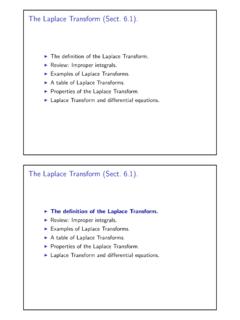
The Laplace Transform (Sect. 6.1). - users.math.msu.edu

The Laplace Transform (Sect. 6.1). I The definition of the Laplace Transform. I Review: Improper integrals. I Examples of Laplace Transforms. I A table of Laplace Transforms. I Properties of the Laplace Transform. I Laplace Transform and differential equations.

  Transform, Laplace transforms, Laplace, The laplace transform

5.1 The Remainder and Factor Theorems.doc; Synthetic Division

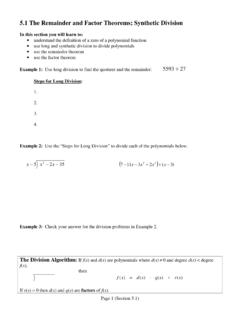
Page 2 (Section 5.1) Example 4: Perform the operation below. Write the remainder as a rational expression (remainder/divisor). 2 1 2 8 2 3 5 4 3 2 + − + + x x x x x Synthetic Division – Generally used for “short” division of polynomials when the divisor is in the form x – c. (Refer to page 506 in your textbook for more examples.)

  Factors, Theorem, Remainder, The remainder and factor theorems

Convolution solutions (Sect. 6.6). - users.math.msu.edu

Convolution solutions (Sect. 6.6). I Convolution of two functions. I Properties of convolutions. I Laplace Transform of a convolution. I Impulse response solution. I Solution decomposition theorem.

Math 133 Series Sequences and series. fa g

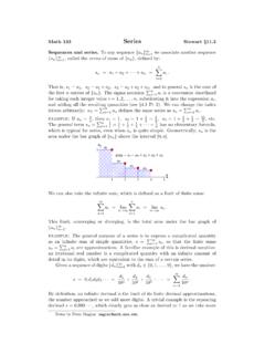
Geometric sequences and series. A general geometric sequence starts with an initial value a 1 = c, and subsequent terms are multiplied by the ratio r, so that a n = ra n 1; explicitly, a n = crn 1. The same trick as above gives a formula for the corresponding geometric series. We have s …

  Series, Sequence, Geometric, Geometric sequences and series, Geometric series, Series sequences and series

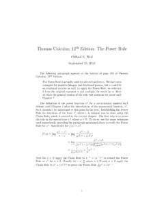
Thomas Calculus; 12th Edition: The Power Rule

Thomas Calculus; 12th Edition: The Power Rule Cli ord E. Weil September 15, 2010 The following paragraph appears at the bottom of page 116 of Thomas Calculus, 12th Edition. The Power Rule is actually valid for all real numbers n.

  Power, Edition, Thomas, Calculus, The power, 12th, Thomas calculus 12th edition, 12th edition, Thomas calculus

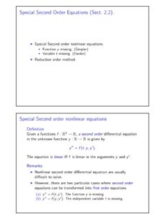
Special Second Order Equations (Sect. 2.2). Special Second ...

Special Second Order Equations (Sect. 2.2). I Special Second order nonlinear equations. I Function y missing. (Simpler) I Variable t missing. (Harder) I Reduction order method. Special Second order nonlinear equations Definition Given a functions f : R3 → R, a second order differential equation in the unknown function y : R → R is given by

  Second, Special, Order, Equations, Sect, Second order, Special second order equations, Special second order

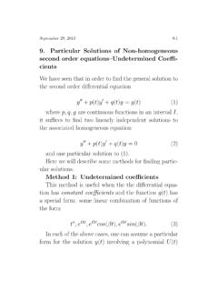
second order equations{Undetermined Coe - cients

September 29, 2013 9-1 9. Particular Solutions of Non-homogeneous second order equations{Undetermined Coe -cients We have seen that in order to nd the general solution to

  Second, Order, Equations, Undetermined, Second order equations undetermined

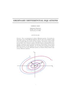
ORDINARY DIFFERENTIAL EQUATIONS

The equations in examples (c) and (d) are called partial di erential equations (PDE), since the unknown function depends on two or more independent variables, t, x, y, and zin these examples, and their partial derivatives appear in the equations.

  Differential, Equations, Variable, Ordinary, Ordinary differential equations

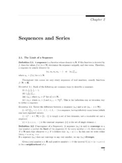
Sequences and Series - Michigan State University

2 2. Sequences and Series A topological way to say lima n = ais the following: Given any -neighborhood V (a) of a, there exists a place in the sequence after which all of the terms are in V (a): Easy Fact: lim(c) = cfor all constant sequences (c): Quanti ers. The de nition of lima n = aquanti es the closeness of a n to aby an arbi-

  Series, Sequence, Sequences and series

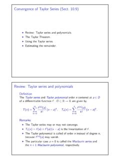
Convergence of Taylor Series (Sect. 10.9) Review: Taylor ...

Convergence of Taylor Series (Sect. 10.9) I Review: Taylor series and polynomials. I The Taylor Theorem. I Using the Taylor series. I Estimating the remainder. The Taylor Theorem Remark: The Taylor polynomial and Taylor series are obtained from a generalization of the Mean Value Theorem: If f : [a,b] → R is differentiable, then there exits c ∈ (a,b) such that

  Review, Convergence

The Gauss-Jordan Elimination Algorithm

Echelon Forms Reduced Row Echelon Form De nition A matrix A is said to be in reduced row echelon form if it is in row echelon form, and additionally it satis es the following two properties: 1 In any given nonzero row, the leading entry is equal to 1, 2 The leading entries are the only nonzero entries in their columns.

  Form, Elimination, Algorithm, Jordan, Gauss, Echelon, The gauss jordan elimination algorithm, Row echelon form

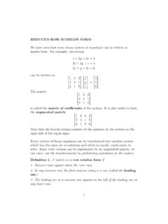
REDUCED ROW ECHELON FORM - United States Naval …

De nition 1. A matrix is in row echelon form if 1. Nonzero rows appear above the zero rows. 2. In any nonzero row, the rst nonzero entry is a one (called the leading one). 3. The leading one in a nonzero row appears to the left of the leading one in any lower row. 1

  Form, United, States, Naval, Reduced, United states naval, Echelon, Reduced row echelon form, Row echelon form

1.3 Solving Systems of Linear Equations: Gauss-Jordan ...

In order to solve a system, we want to \reduce" the augmented matrix to a form where we can easily identify the solution. This form is called \reduced-row echelon form." It is equivalent to the original system, but simpli ed. The method by which we simplify an augmented matrix to its reduced form is called the Gauss-Jordan Elimination Method.

  Form, Echelon, Row echelon form

DIFFERENTIAL EQUATIONS PRACTICE PROBLEMS: ANSWERS

10. The reduced row echelon form for the matrix Abelow has been computed by Matlab: A= 2 −4 −12 −36 1−5 5 −10 −4 −1 rref(A)= 1 −203 00 14 00 00 Use this to find all solutions of 2x1 −4x2 −x3 =2 −3x1 +6x2 +x3 = −5 5x1 −10x2 −4x3 = −1 and express your answer in vector form.

  Form, Echelon, Row echelon form

4 Span and subspace - Auburn University

that x2 is not a multiple of x1 so the row echelon form of the corresponding augmented matrix will have a pivot in each row and hence no pivot in the augmented column.) On the other hand, if x1 and x2 are parallel and nonzero, then both vectors lie on the same line through the origin and Span{x1,x2} is this line. (In this

  Form, Span, Subspaces, Echelon, 4 span and subspace, Row echelon form

Row Echelon Form and Number of Solutions

Row Echelon Form and Number of Solutions 1. Row Echelon Form In these notes we will de ne one of the most important forms of a matrix. It is one of the \easier" forms of a system to solve, in particular, only back-substitution is needed to complete the solution of …

  Form, Echelon, Row echelon form

Matrix Solutions to Linear Equations - Alamo Colleges …

Our reduced row-echelon matrix will look like . 10 0 01 0 001 a b c ⎡⎤ ⎢⎥ ⎢⎥ ⎢⎥⎣⎦ where a, b, and c are the solutions for the three variables. The reduced row-echelon matrix will generally be in the form above, containing only 1’s and 0’s to the left of the vertical line, with the 1’s in a diagonal pattern extending ...

  Form, Linear, Solutions, College, Equations, Matrix, Omala, Echelon, Matrix solutions to linear equations, Alamo colleges

4.5 Solve Systems of Equations Using Matrices

Aug 04, 2018 · Using row operations, get zeros in column 1 below the 1. Continue the process until the matrix is in row-echelon form. Multiply row 2 by −2 and add it to row 3. At this point, we have all zeros in the bottom row. Write the corresponding system of …

  Form, Echelon, Row echelon form

MATH 304 Linear Algebra Lecture 11: Basis and dimension.

of the form r1w1+r2w2+r3w3+r4w4 = 0, where ri ∈ R are not all equal to zero. Equivalently, 1 0 2 1 1 1 3 1 0 1 1 1 r1 r2 r3 r4 = 0 0 0 . To solve this system …

  Form