Transcription of FINITE ELEMENT ANALYSIS SIMPLY EXPLAINED
1 FINITE ELEMENT ANALYSIS SIMPLY EXPLAINED T. C. Kennedy Oregon State University July 2016 2 1. INTRODUCTION This article is written for engineers who want to understand how FINITE ELEMENT ANALYSIS works but are not interested in developing a level of proficiency that would allow them to perform such an ANALYSIS themselves. Purists may find many of the explanations to be over-simplified. If this is a concern, you should stop reading now. FINITE ELEMENT ANALYSIS was originally developed for analyzing complex structures. It is currently used to analyze a variety of physical systems including heat transfer, fluid mechanics, magnetism, etc.
2 However, from an intuitive standpoint, the basic ideas are most easily developed using solid mechanics concepts. Most engineering curricula include a course on elementary mechanics of materials. Thus, we will use those concepts as building blocks to illustrate the process. A brief review of some of these basic concepts and matrix mathematics is presented next. Elementary Mechanics of Materials Mechanics of Materials deals with simple structures that deform under load. A body is considered to be in equilibrium when the following is satisfied: 0xF 0intApoxM 0yF 0intApoyM (1-1) 0zF 0intApozM , when the net forces in the x, y, and z-directions are zero, and the net moments in the x,y, and z-directions about some reference point A are zero.
3 The effect of applying external loads to a body is to cause stress inside the body. The stresses at an internal point can be represented on the faces of a small cube around the point as shown in Figure 1-1. Figure 1-1 3 Note that on each face, there is one component of normal stress acting perpendicular to the face and two components of shear stress acting tangent to the face. The effect of the normal stress is to cause the body to stretch in the direction of the stress and to shrink in the two directions perpendicular to the stress. These deformations can be described by strains (elongation per unit length).
4 The normal strains in the x, y, and z-directions ( x, y, z) are related to the normal stresses ( x, y, z ) through Hooke s law as follows: )]([1zyxxE )]([1zxyyE (1-2) )]([1yxzzE where E is Young s modulus (or elastic modulus), and is Poisson s ratio. E and are material properties. The effect of the shear stress is to cause a shear strain which represents the change in angle (in radians) between the sides of the cube to something smaller or larger than the original right angle. The shear strains ( xy, xz, yz) are related to the shear stresses ( xy, xz, yz,) as follows: Gxyxy/ Gxzxz/ (1-3) Gyzyz/ where G is the shear modulus and G=E/(1+2v).
5 The simple definition of normal strain as stretch per unit length is inconvenient for cases where the strain is not uniform throughout the body. In three dimensions each point on the body will have displacements in the x, y, and z-directions (u, v, and w, respectively). The Theory of Elasticity provides relations between the components of strain and the displacements as xux yvy zwz (1-4) xvyuxy xwzuxz ywzvyz (1-5) Simultaneous Equations and Matrices Solving simultaneously linear algebraic equations is a routine task for a computer. Therefore, we are motivated to reduce the mathematics of our physical problem to a set of simultaneous equations.
6 Let's consider the following set of equations 1062 yx (1-6) 853 yx (1-7) 4 where x and y are unknowns. We can rewrite these in matrix format as follows: 8105362yx (1-8) On the left side of the equation, the terms in the row of the first matrix are multiplied by the terms in the columns of the second matrix to recover the original equations. We will find it convenient to use matrix methods to set up the equations for our physical problem for computer solution. 2. MATRIX STRUCTURAL ANALYSIS Many of the techniques in the FINITE ELEMENT procedure are common to those of matrix structural ANALYSIS . Therefore, we will review some of these basic concepts.
7 Spring Structures We begin with the ANALYSIS of a very simple structure composed of springs (for example , see Figure 2-1). Figure 2-1 Although these structures are not particularly interesting in a practical sense, their simplicity allows for transparency in the mathematics. Spring ELEMENT Let's consider a simple spring where loads fi and fj may be applied to its endpoints (which we will call nodes) and give them the labels i and j as shown in Figure 2-2. Figure 2-2 When this spring is part of a larger spring structure, we will be interested in the displacements of its node points ui and uj. We will use the sign convention that forces and displacements that act to the right are positive and those to the left are negative.
8 Before determining the relationship between the nodal forces fi and fj and nodal displacements ui and uj, we will use our knowledge that the stretch of the spring must be proportional to the force and vice versa. Therefore, these quantities must be related mathematically as follows ijijiiifuKuK (2-1) jjjjijifuKuK (2-2) 5 where Kii, Kij, Kji, and Kjj are constants. We will determine these constants by considering two special cases. In the first case we let uj=0. Then, the equations give iiiifuK (2-3) jijifuK (2-4) Physically, we have the situation shown in Figure 2-3. Figure 2-3 The force in the spring is fi and the compression of the spring is ui.
9 From the spring law we know iikuf (2-5) where k is the spring constant. Comparing this to equation (2-3), we conclude kKii (2-6) The reaction force at node j must be equal and opposite to that at node i. Therefore, iijkuff (2-7) Comparing this to equation (2-4) we conclude that kKji (2-8) For the second case, we set ui=0 . Then the equations (2-1) and (2-2) give ijijfuK (2-9) jjjjfuK (2-10) Physically, we have the situation shown in Figure 2-4. Figure 2-4 The force in the spring is fj, and the stretch of the spring is uj . Therefore, the spring law gives jjkuf (2-11) Comparing this to equation (2-10), we conclude kKjj (2-12) The reaction force at node i is equal and opposite to that at node j.
10 Therefore, jjikuff (2-13) Comparing this to equation (2-9) gives kKij (2-14) Now that each K has been determined, we can write equations (2-1) and (2-2) as ijifkuku (2-15) jjifkuku (2-16) Rewriting this in matrix form gives 6 jijiffuukkkk (2-17) The first matrix in the equation above is called the ELEMENT stiffness matrix. As we will see in the next section, we can use this matrix as a building block to determine the equations relating displacements to forces in a system with any number of springs. System of springs Let us now consider a spring structure composed of two springs a and b with spring constants ka and kb as shown in Figure 2-5.