Transcription of Introduction to Queueing Theory
1 Introduction to Queueing Theory Raj Jain Washington University in Saint Louis or A Mini-Course offered at UC Berkeley, Sept-Oct 2012. These slides and audio/video recordings are available on-line at: and ~jain/queue UC Berkeley, Fall 2012 2012 Raj Jain 30-1. Overview Queueing Notation Rules for All Queues Little's Law Types of stochastic Processes UC Berkeley, Fall 2012 2012 Raj Jain 30-2. Basic Components of a Queue 1. Arrival 6. Service 2. Service time process discipline distribution 5. Population Size 4. Waiting positions 3. Number of servers UC Berkeley, Fall 2012 2012 Raj Jain 30-3. Kendall Notation A/S/m/B/K/SD. A: Arrival process S: Service time distribution m: Number of servers B: Number of buffers (system capacity). K: Population size, and SD: Service discipline UC Berkeley, Fall 2012 2012 Raj Jain 30-4.
2 Arrival Process Arrival times: Interarrival times: j form a sequence of Independent and Identically Distributed (IID) random variables Notation: M = Memoryless Exponential E = Erlang H = Hyper-exponential D = Deterministic constant G = General Results valid for all distributions UC Berkeley, Fall 2012 2012 Raj Jain 30-5. Service Time Distribution Time each student spends at the terminal. Service times are IID. Distribution: M, E, H, D, or G. Device = Service center = Queue Buffer = Waiting positions UC Berkeley, Fall 2012 2012 Raj Jain 30-6. Service Disciplines First-Come-First-Served (FCFS). Last-Come-First-Served (LCFS) = Stack (used in 9-1-1 calls). Last-Come-First-Served with Preempt and Resume (LCFS-PR). Round-Robin (RR) with a fixed quantum. Small Quantum Processor Sharing (PS). Infinite Server: (IS) = fixed delay Shortest Processing Time first (SPT).
3 Shortest Remaining Processing Time first (SRPT). Shortest Expected Processing Time first (SEPT). Shortest Expected Remaining Processing Time first (SERPT). Biggest-In-First-Served (BIFS). Loudest-Voice-First-Served (LVFS). UC Berkeley, Fall 2012 2012 Raj Jain 30-7. Example M/M/3/20/1500/FCFS. Time between successive arrivals is exponentially distributed. Service times are exponentially distributed. Three servers 20 Buffers = 3 service + 17 waiting After 20, all arriving jobs are lost Total of 1500 jobs that can be serviced. Service discipline is first-come-first-served. Defaults: Infinite buffer capacity Infinite population size FCFS service discipline. G/G/1 = G/G/1/ / /FCFS. UC Berkeley, Fall 2012 2012 Raj Jain 30-8. Quiz 30A. Key: A/S/m/B/K/SD. TF. The number of servers in a M/M/1/3 queue is 3. G/G/1/30/300/LCFS queue is like a stack M/D/3/30 queue has 30 buffers G/G/1 queue has population size D/D/1 queue has FCFS discipline UC Berkeley, Fall 2012 2012 Raj Jain 30-9.
4 Exponential Distribution Probability Density Function (pdf): 1. a 1 x/a f(x). f (x) = e a Cumulative Distribution x Z xFunction (cdf): 1. F (x) = P (X < x) = f (x)dx = 1 e x/a 0 F(x). Mean: a x Variance: a2. Coefficient of Variation = (Std Deviation)/mean = 1. Memoryless: Expected time to the next arrival is always a regardless of the time since the last arrival Remembering the past history does not help. UC Berkeley, Fall 2012 2012 Raj Jain 30-11. Erlang Distribution Sum of k exponential random variables 1 k Series of k servers with exponential service times Xk X= xi where xi exponential i=1. Probability Density Function (pdf): xk 1 e x/a f (x) =. (k 1)!ak Expected Value: ak Variance: a2k CoV: 1/ k UC Berkeley, Fall 2012 2012 Raj Jain 30-12. Hyper-Exponential Distribution The variable takes ith value with probability pi x1.
5 X x2.. xm xi is exponentially distributed with mean ai Higher variance than exponential Coefficient of variation > 1. UC Berkeley, Fall 2012 2012 Raj Jain 30-13. Group Arrivals/Service Bulk arrivals/service M[x]: x represents the group size G[x]: a bulk arrival or service process with general inter-group times. Examples: M[x]/M/1 : Single server queue with bulk Poisson arrivals and exponential service times M/G[x]/m: Poisson arrival process, bulk service with general service time distribution, and m servers. UC Berkeley, Fall 2012 2012 Raj Jain 30-14. Quiz 30B. Exponential distribution is denoted as ___. _____ distribution represents a set of parallel exponential servers Erlang distribution Ek with k=1 is same as _____. distribution UC Berkeley, Fall 2012 2012 Raj Jain 30-15. Key Variables 1. 2.. m nq ns n Previous Begin End Arrival Arrival Service Service Time w s r UC Berkeley, Fall 2012 2012 Raj Jain 30-17.
6 Key Variables (cont). Inter-arrival time = time between two successive arrivals. Mean arrival rate = 1/E[ ]. May be a function of the state of the system, , number of jobs already in the system. s = Service time per job. = Mean service rate per server = 1/E[s]. Total service rate for m servers is m . n = Number of jobs in the system. This is also called queue length. Note: Queue length includes jobs currently receiving service as well as those waiting in the queue. UC Berkeley, Fall 2012 2012 Raj Jain 30-18. Key Variables (cont). nq = Number of jobs waiting ns = Number of jobs receiving service r = Response time or the time in the system = time waiting + time receiving service w = Waiting time = Time between arrival and beginning of service UC Berkeley, Fall 2012 2012 Raj Jain 30-19. Rules for All Queues Rules: The following apply to G/G/m queues 1.
7 Stability Condition: Arrival rate must be less than service rate < m . Finite-population or finite-buffer systems are always stable. Instability = infinite queue Sufficient but not necessary. D/D/1 queue is stable at = . 2. Number in System versus Number in Queue: n = nq+ ns Notice that n, nq, and ns are random variables. E[n]=E[nq]+E[ns]. If the service rate is independent of the number in the queue, Cov(nq,ns) = 0. UC Berkeley, Fall 2012 2012 Raj Jain 30-20. Rules for All Queues (cont). 3. Number versus Time: If jobs are not lost due to insufficient buffers, Mean number of jobs in the system = Arrival rate Mean response time 4. Similarly, Mean number of jobs in the queue = Arrival rate Mean waiting time This is known as Little's law. 5. Time in System versus Time in Queue r=w+s r, w, and s are random variables.
8 E[r] = E[w] + E[s]. UC Berkeley, Fall 2012 2012 Raj Jain 30-21. Rules for All Queues(cont). 6. If the service rate is independent of the number of jobs in the queue, Cov(w,s)=0. UC Berkeley, Fall 2012 2012 Raj Jain 30-22. Quiz 30C. If a queue has 2 persons waiting for service, the number is system is ____. If the arrival rate is 2 jobs/second, the mean inter- arrival time is _____ second. In a 3 server queue, the jobs arrive at the rate of 1. jobs/second, the service time should be less than ____. second/job for the queue to be stable. UC Berkeley, Fall 2012 2012 Raj Jain 30-23. Little's Law Mean number in the system = Arrival rate Mean response time This relationship applies to all systems or parts of systems in which the number of jobs entering the system is equal to those completing service. Named after Little (1961).
9 Based on a black-box view of the system: Arrivals Black Departures Box In systems in which some jobs are lost due to finite buffers, the law can be applied to the part of the system consisting of the waiting and serving positions UC Berkeley, Fall 2012 2012 Raj Jain 30-25. Proof of Little's Law 4 Arrival 4. Job 3 Number 3. number in 2 2. Departure System 1 1. 12345678 12345678. Time Time If T is large, arrivals = departures = N 4. Arrival rate = Total arrivals/Total time= N/T Time 3. Hatched areas = total time spent inside the in system by all jobs = J 2. System Mean time in the system= J/N 1. Mean Number in the system = J/T = 1 2 3. Job number = Arrival rate Mean time in the system UC Berkeley, Fall 2012 2012 Raj Jain 30-26. Application of Little's Law Arrivals Departures Applying to just the waiting facility of a service center Mean number in the queue = Arrival rate Mean waiting time Similarly, for those currently receiving the service, we have: Mean number in service = Arrival rate Mean service time UC Berkeley, Fall 2012 2012 Raj Jain 30-27.
10 Example A monitor on a disk server showed that the average time to satisfy an I/O request was 100 milliseconds. The I/O rate was about 100 requests per second. What was the mean number of requests at the disk server? Using Little's law: Mean number in the disk server = Arrival rate Response time = 100 (requests/second) ( seconds). = 10 requests UC Berkeley, Fall 2012 2012 Raj Jain 30-28. Quiz 30D. Key: n = R. During a 1 minute observation, a server received 120. requests. The mean response time was 1 second. The mean number of queries in the server is _____. UC Berkeley, Fall 2012 2012 Raj Jain 30-29. stochastic Processes Process: Function of time stochastic Process: Random variables, which are functions of time Example 1: n(t) = number of jobs at the CPU of a computer system Take several identical systems and observe n(t).