Transcription of Lecture 1 ELE 301: Signals and Systems - Princeton University
1 Lecture 1. ELE 301: Signals and Systems Prof. Paul Cuff Princeton University Fall 2011-12. Cuff ( Lecture 1) ELE 301: Signals and Systems Fall 2011-12 1 / 45. Course Overview Time-Series Representation of Signals Typically think of a signal as a time series , or a sequence of values in time f(t). t Useful for saying what is happening at a particular time Not so useful for capturing the overall characteristics of the signal . Cuff ( Lecture 1) ELE 301: Signals and Systems Fall 2011-12 2 / 45. Idea 1: Frequency Domain Representation of Signals Represent signal as a combination of sinusoids 1. Amplitude sin( 1t). 0. !1. 0 1. Time, t 1. sin( 2t). Amplitude 0. !1. 0 1. Time, t 1. sin( 3t). Amplitude 0. !1. 0 1. Time, t 1. Amplitude 0. !1. 0 1. Time, t f (t) = sin( 1t) + sin( 2t) + sin( 3t). Cuff ( Lecture 1) ELE 301: Signals and Systems Fall 2011-12 3 / 45. This example is mostly a sinusoid at frequency 2 , with small contributions from sinusoids at frequencies 1 and 3.
2 I Very simple representation (for this case). I Not immediately obvious what the value is at any particular time. Why use frequency domain representation? I Simpler for many types of Signals (AM radio signal , for example). I Many Systems are easier to analyze from this perspective (Linear Systems ). I Reveals the fundamental characteristics of a system. Rapidly becomes an alternate way of thinking about the world. Cuff ( Lecture 1) ELE 301: Signals and Systems Fall 2011-12 4 / 45. Demonstration: Piano Chord You are already a high sophisticated system for performing spectral analysis! Listen to the piano chord. You hear several notes being struck, and fading away. This is waveform is plotted below: Amplitude 0. 0 1 2 3 Time, seconds Amplitude 0. Time, seconds Cuff ( Lecture 1) ELE 301: Signals and Systems Fall 2011-12 5 / 45. The time series plot shows the time the chord starts, and its decay, but it is difficult tell what the notes are from the waveform.
3 If we represent the waveform as a sum of sinusoids at different frequencies, and plot the amplitude at each frequency, the plot is much simpler to understand. 40. 30. Magnitude 20. 10. 0. 5000 4000 3000 2000 1000 0 1000 2000 3000 4000 5000. Frequency, Hz 40. 30. Magnitude 20. 10. 0. 0 500 1000 1500. Frequency, Hz Cuff ( Lecture 1) ELE 301: Signals and Systems Fall 2011-12 6 / 45. Idea 2: Linear Systems are Easy to Analyze for Sinusoids Example: We want to predict what will happen when we drive a car over a curb. The curb can be modelled as a step input. The dynamics of the car are governed by a set of differential equations, which are hard to solve for an arbitrary input (this is a linear system). Input: Curb Car Dynamics Output Differential ? Equations Hard to Solve Directly Cuff ( Lecture 1) ELE 301: Signals and Systems Fall 2011-12 7 / 45. After transforming the input and the differential equations into the frequency domain, Input: Curb Car Dynamics Output Differential Equations Frequency Frequency Transfer Domain Function Domain Input Output Easy to Solve, Multiplication Frequency Domain Solving for the frequency domain output is easy.
4 The time domain output is found by the inverse transform. We can predict what happens to the system. Cuff ( Lecture 1) ELE 301: Signals and Systems Fall 2011-12 8 / 45. Idea 3: Frequency Domain Lets You Control Linear Systems Often we want a system to do something in particular automatically I Airplane to fly level I Car to go at constant speed I Room to remain at a constant temperature This is not as trivial as you might think! Cuff ( Lecture 1) ELE 301: Signals and Systems Fall 2011-12 9 / 45. Example: Controlling a car's speed. Applying more gas causes the car to speed up gas speed Car Normally you close the loop . gas speed Car You How can you do this automatically? Cuff ( Lecture 1) ELE 301: Signals and Systems Fall 2011-12 10 / 45. Use feedback by comparing the measured speed to the requested speed: requested speed error gas speed + + k Car - This can easily do something you don't want or expect, and oscillate out of control.
5 Frequency domain analysis explains why, and tells you how to design the system to do what you want. Cuff ( Lecture 1) ELE 301: Signals and Systems Fall 2011-12 11 / 45. Course Outline It is useful to represent Signals as sums of sinusoids (the frequency domain). This is the correct domain to analyze linear time-invariant Systems Linear feedback control, sampling, modulation, etc. What sort of Signals and Systems are we talking about? Cuff ( Lecture 1) ELE 301: Signals and Systems Fall 2011-12 12 / 45. Signals Typical think of Signals in terms of communication and information I radio signal I broadcast or cable TV. I audio I electric voltage or current in a circuit More generally, any physical or abstract quantity that can be measured, or influences one that can be measured, can be thought of as a signal . I tension on bike brake cable I roll rate of a spacecraft I concentration of an enzyme in a cell I the price of dollars in euros I the federal deficit Very general concept.
6 Cuff ( Lecture 1) ELE 301: Signals and Systems Fall 2011-12 13 / 45. Systems Typical Systems take a signal and convert it into another signal , I radio receiver I audio amplifier I modem I microphone I cell telephone I cellular metabolism I national and global economies Internally, a system may contain many different types of Signals . The Systems perspective allows you to consider all of these together. In general, a system transforms input Signals into output Signals . Cuff ( Lecture 1) ELE 301: Signals and Systems Fall 2011-12 14 / 45. Continuous and discrete Time Signals Most of the Signals we will talk about are functions of time. There are many ways to classify Signals . This class is organized according to whether the Signals are continuous in time, or discrete . A continuous-time signal has values for all points in time in some (possibly infinite) interval. A discrete time signal has values for only discrete points in time.
7 F(t) f [n]. -4 -2 0 2 4. t n Signals can also be a function of space (images) or of space and time (video), and may be continuous or discrete in each dimension. Cuff ( Lecture 1) ELE 301: Signals and Systems Fall 2011-12 15 / 45. Types of Systems Systems are classified according to the types of input and output Signals Continuous-time system has continuous-time inputs and outputs. I AM or FM radio I Conventional (all mechanical) car discrete -time system has discrete -time inputs and outputs. I PC computer game I Matlab I Your mortgage Hybrid Systems are also very important (A/D, D/A converters). I You playing a game on a PC. I Modern cars with ECU (electronic control units). I Most commercial and military aircraft Cuff ( Lecture 1) ELE 301: Signals and Systems Fall 2011-12 16 / 45. Continuous Time Signals Function of a time variable, something like t, , t1 . The entire signal is denoted as v , v (.), or v (t), where t is a dummy variable.
8 The value of the signal at a particular time is v ( ), or v (t), t = 2. p(t), Pa 1. 0. 1 2 3 t, us -1 Ultrasound Pulse Cuff ( Lecture 1) ELE 301: Signals and Systems Fall 2011-12 17 / 45. discrete Time Signals Fundamentally, a discrete -time signal is sequence of samples, written x[n]. where n is an integer over some (possibly infinite) interval. Often, at least conceptually, samples of a continuous time signal x[n] = x(nT ). where n is an integer, and T is the sampling period. x[n]. -4 -2 0 2 4. n discrete time Signals may not represent uniform time samples (NYSE. closes, for example). There may1) not be an underlying Cuff ( Lecture continuous ELE 301: Signals and Systems time signal (NYSE. Fall 2011-12 closes, 18 / 45. Summary A signal is a collection of data Systems act on Signals (inputs and outputs). Mathematically, they are similar. A signal can be represented by a function. A system can be represented by a function (the domain is the space of input Signals ).)
9 We focus on 1-dimensional Signals . Our Systems are not random. Cuff ( Lecture 1) ELE 301: Signals and Systems Fall 2011-12 19 / 45. signal Characteristics and Models Operations on the time dependence of a signal I Time scaling I Time reversal I Time shift I Combinations signal characteristics Periodic Signals Complex Signals Signals sizes signal Energy and Power Cuff ( Lecture 1) ELE 301: Signals and Systems Fall 2011-12 20 / 45. Amplitude Scaling The scaled signal ax(t) is x(t) multiplied by the constant a 2 2. 1 1 2x(t). x(t). -2 -1 0 1 2 -2 -1 0 1 2. t The scaled signal ax[n] is x[n] multiplied by the constant a 2 x[n] 2 2x[n]. 1 1. -2 -1 0 1 2 n -2 -1 0 1 2 n Cuff ( Lecture 1) ELE 301: Signals and Systems Fall 2011-12 21 / 45. Time Scaling, Continuous Time A signal x(t) is scaled in time by multiplying the time variable by a positive constant b, to produce x(bt). A positive factor of b either expands (0 < b < 1) or compresses (b > 1) the signal in time.
10 2 2. b=1 b=2. 1. x(t) 1 x(2t). b = 1/2 2. 1 x(t/2). -2 -1 0 1 2 -2 -1 0 1 2. t t -3 -2 -1 0 1 2 3 t Cuff ( Lecture 1) ELE 301: Signals and Systems Fall 2011-12 22 / 45. Time Scaling, discrete Time The discrete -time sequence x[n] is compressed in time by multiplying the index n by an integer k, to produce the time-scaled sequence x[nk]. This extracts every k th sample of x[n]. Intermediate samples are lost. The sequence is shorter. x[n] y[n] = x[2n]. -4 -3 -2 -1 0 1 2 3 4 -2 -1 0 1 2. n n Called downsampling, or decimation. Cuff ( Lecture 1) ELE 301: Signals and Systems Fall 2011-12 23 / 45. The discrete -time sequence x[n] is expanded in time by dividing the index n by an integer m, to produce the time-scaled sequence x[n/m]. This specifies every mth sample. The intermediate samples must be synthesized (set to zero, or interpolated). The sequence is longer. x[n] y[n] = x[n/2]. -2 -1 0 1 2 -4 -3 -2 -1 0 1 2 3 4. n n Called upsampling, or interpolation.