Transcription of Non-Linear & Logistic Regression
1 Non-Linear & Logistic Regression If the statistics are boring, then you've got the wrong numbers. Edward R. Tufte (Statistics Professor, Yale University) Regression Analyses When do we use these? PART 1: find a relationship between response variable (Y) and a predictor variable (X) ( Y~X) PART 2: use relationship to predict Y from X Simple linear Regression : y = b + m*x y = 0 + 1 * x1 Multiple linear Regression : y = 0 + 1*x1 + 2*x2 .. + n*xn Non linear Regression : when a line just doesn t fit our data Logistic Regression : when our data is binary (data is represented as 0 or 1) Non-Linear Regression Curvilinear relationship between response and predictor variables The right type of Non-Linear model are usually conceptually determined based on biological considerations For a starting point we can plot the relationship between the 2 variables and visually check which model might be a good option There are obviously MANY curves you can generate to try and fit your data Exponential Curve Non-Linear Regression option #1 Rapid increasing/decreasing change in Y or X for a change in the other Ex: bacteria growth/decay, human population growth, infection rates (humans, trees, etc.)
2 : = + predictor (x) response (y) predictor (x) response (y) predictor (x) response (y) predictor (x) response (y) a a a a 0 < c < 1 +b c > 1 +b 0 < c < 1 -b c > 1 -b : = + Logarithmic Curve Non-Linear Regression option #2 Rapid increasing/decreasing change in Y or X for a change in the other Ex: survival thresholds, resource optimization predictor (x) response (y) predictor (x) response (y) predictor (x) response (y) predictor (x) response (y) a a a a -c +b +c +b -c -b +c -b Hyperbolic Curve Non-Linear Regression option #3 Rapid increasing/decreasing change in Y or X for a change in the other Ex: survival of a function of population Similar to exponential and logarithmic curve but now we have 2 asymptotes : = + + predictor (x) response (y) predictor (x) response (y) a c +b a c -b Parabolic Curve Non-Linear Regression option #4 Rapid increasing/decreasing change in Y or X for a change in the other followed by the reverse trend Ex: survival of a function of an environmental variable : = + 2 predictor (x) response (y) predictor (x) response (y) a c +b a c -b Upward Parabolic Downward Parabolic Gaussian Curve Non-Linear Regression option #5 Resembles a normal distribution Ex: survival of a function of an environmental variable Where 0 < b < 1 : = 2 predictor (x) response (y) b a c Sigmoidal Curve Non-Linear Regression option #6 Stability in Y followed by rapid increase then stability again Ex: restricted growth, learning response, a threshold has to occur for a response effect Where b > 1 and c > 1 : = 1+ + predictor (x) response (y) b a c d Michaelis Menten Curve Non-Linear Regression option #7.
3 = + predictor (x) response (y) predictor (x) response (y) 12 a Rapid increasing/decreasing change in Y or X for a change in the other Ex: biological process as a function of resource availability Similar to exponential and logarithmic curve but now we have 2 parameters this model comes from kinetics/physiology a b a -b Non-Linear Regression Curve Fitting Procedure: your variables to visualize the relationship curve does the pattern resemble? might alternative options be? on the curves you want to compare and run a Non-Linear Regression curve fitting will have to estimate your parameters from your curve to have starting values for your curve fitting function you have parameters for your curves compare models with AIC the model with the lowest AIC on your point data to visualize fit Non-Linear Regression curve fitting in R: (" ") nlsLM(responseY~MODEL, start=list(starting values for model parameters)) Non-Linear Regression Output from R Non-Linear model that we fit Simplified logarithmic with slope=0 Estimates of model parameters Residual sum-of-squares for your Non-Linear model Number of iterations needed to estimate the parameters Non-Linear Regression Curve Fitting Procedure: your variables to visualize the relationship curve does the pattern resemble?
4 Might alternative options be? on the curves you want to compare and run a Non-Linear Regression curve fitting will have to estimate your parameters from your curve to have starting values for your curve fitting function you have parameters for your curves compare models with AIC the model with the lowest AIC on your point data to visualize fit Non-Linear Regression curve fitting in R: (" ") nlsLM(responseY~MODEL, start=list(starting values for model parameters)) Akaike s Information Criterion (AIC) How do we decide which model is best? AIC considers both the fit of the model and the model complexity Complexity is measured as number parameters or the use of higher order polynomials Allows us to balance over- and under-fitting in our modelled relationships We want a model that is as simple as possible, but no simpler A reasonable amount of explanatory power is traded off against model complexity AIC measures the balance of this for us Hirotugu Akaike, 1927-2009 In the 1970s he used information theory to build a numerical equivalent of Occam's razor Occam s razor: All else being equal, the simplest explanation is the best one For model selection, this means the simplest model is preferred to a more complex one Of course, this needs to be weighed against the ability of the model to actually predict anything Akaike s Information Criterion (AIC) AIC in R Akaike s Information Criterion in R to determine best model.
5 AIC(nlsLM(responseY~MODEL1, start=list(starting values))) AIC(nlsLM(responseY~MODEL2, start=list(starting values))) AIC(nlsLM(responseY~MODEL3, start=list(starting values))) AIC is useful because it can be calculated for any kind of model allowing comparisons across different modelling approaches and model fitting techniques Model with the lowest AIC value is the model that fits your data best ( minimizes your model residuals) Output from R is a single AIC value Non-Linear Regression Curve fitting Use the parameter estimates outputted from nlsLM() to generate curve for plotting Non-Linear Regression NLR make no assumptions for normality, equal variances, or outliers However the assumptions of independence (spatial & temporal) and design considerations (randomization, sufficient replicates, no pseudoreplication) still apply We don t have to worry about statistical power here because we are fitting relationships All we care about is if or how well we can model the relationship between our response and predictor variables Assumptions Non-Linear Regression Calculating an R2 is NOT APPROPIATE for Non-Linear Regression Why?
6 For linear models, the sums of the squared errors always add up in a specific manner: + = Therefore 2= which mathematically must produce a value between 0 and 100% But in nonlinear Regression + Therefore the ratio used to construct R2 is bias in nonlinear Regression Best to use AIC value and the measurement of the residual sum-of-squares to pick best model then plot the curve to visualize the fit R2 for goodness of fit Logistic Regression ( logit Regression ) Relationship between a binary response variable and predictor variables Binary response variable can be considered a class (1 or 0) Yes or No Present or Absent The linear part of the Logistic Regression equation is used to find the probability of being in a category based on the combination of predictors Predictor variables are usually (but not necessarily) continuous But it is harder to make inferences from Regression outputs that use discrete or categorical variables.
7 = 0+ 1 1+ 2 2+ + 1 0+ 1 1+ 2 2+ + Logit Model Binomial distribution vs Normal distribution Key difference: Values are continuous (Normal) vs discrete (Binomial) As sample size increases the binomial distribution appears to resemble the normal distribution Binomial distribution is a family of distributions because the shape references both the number of observations and the probability of getting a success - a value of 1 What is probability of x success in n independent and identically distributed Bernoulli trials? Bernoulli trial (or binomial trial) - a random experiment with exactly two possible outcomes, "success" and "failure", in which the probability of success is the same every time the experiment is conducted Linear Regression -references the Gaussian (normal) distribution -uses ordinary least squares to find a best fitting line the estimates parameters that predict the change in the dependent variable for change in the independent variable Logistic Regression -references the Binomial distribution -estimates the probability (p) of an event occurring (y=1) rather then not occurring (y=0) from a knowledge of relevant independent variables (our data) - Regression coefficients are estimated using maximum likelihood estimation (iterative process)
8 Logistic Regression vs Linear Regression maximum likelihood estimation Complex iterative process to find coefficient values that maximizes the likelihood function likelihood function - probability for the occurrence of a observed set of values X and Y given a function with defined parameters Process: with a tentative solution for each coefficient it slightly to see if the likelihood function can be improved this revision until improvement is minute, at which point the process is said to have converged How coefficients are estimated for Logistic Regression Linear Regression -references the Gaussian (normal) distribution -uses ordinary least squares to find a best fitting line the estimates parameters that predict the change in the dependent variable for change in the independent variable Logistic Regression -references the Binomial distribution -estimates the probability (p) of an event occurring (y=1) rather then not occurring (y=0) from a knowledge of relevant independent variables (our data) - Regression coefficients are estimated using maximum likelihood estimation (iterative process) Logistic Regression vs Linear Regression Simple Logistic Regression in R.
9 Lm(response~predictor, family="binomial") summary(lm(response~predictor, family="binomial")) Multiple Logistic Regression in R: lm(response~predictor1+predictor2+..+pre dictorN, family="binomial") summary(lm(response~predictor1+predictor 2+..+predictorN, family="binomial")) Logistic Regression ( logit Regression ) Output from R Estimate of model parameters (intercept and slope) Standard error of estimates Tests the null hypothesis that the coefficient is equal to zero (no effect) A predictor that has a low p-value is likely to be a meaningful addition to your model because changes in the predictor's value are related to changes in the response variable A large p-value suggests that changes in the predictor are not associated with changes in the response AIC value for the model In linear Regression , the relationship between the dependent and the independent variables is linear However this assumption is not made in Logistic Regression so we cannot use the calculation 2= -REMEMBER we are not using sum-of-squares to estimate our parameters we are using maximum likelihood estimation We can however calculate a pseudo R2 -Lots of options on how to do this, but the best for Logistic Regression appears to be McFadden's calculation Logistic Regression ( logit Regression ) Pseudo R2 for goodness of fit 2=1 = Estimated likelihood Estimating McFadden s pseudo R2 in R.
10 Mod=lm(response~predictor,family="binomi al") $deviance/mod$ NOTE: Pseudo R2 will be MUCH lower than R2 values! Logistic Regression ( logit Regression ) Logistic Regression make no assumptions for normality, equal variances, or outliers However the assumptions of independence (spatial & temporal) and design considerations (randomization, sufficient replicates, no pseudoreplication) still apply Logistic Regression assumes the response variable is binary (0 & 1) We don t have to worry about statistical power here because we are fitting relationships All we care about is if or how well we can model the relationship between our response and predictor variables Assumptions A Non-Linear or Logistic relationship DOES NOT imply causation! AIC or pseudo 2 implies a relationship rather than one or multiple factors causing another factor value Be careful of your interpretations! Important to Remember