Transcription of On Reference RIAA Networks - hagtech.com
1 On Reference RIAA Networks by Jim Hagerman You'd think there would be nothing left to say. Everything you need to know about RIAA Networks has already been published. However, a few years back I came across an interesting chapter in a vacuum tube book[1] which spoke of a mythical s corner in the RIAA response. Huh? That's 50kHz. The seminal works[2][3] never mentioned this, equalization was to appear as Figure 1. Figure 1. Desired inverse RIAA response from Lipshitz. Hmmm. The mythical corner frequency is shown as f4 but ideally should be missing. Or should it? To quote from Allen Wright's book[1].
2 Look back at the graph of the recording EQ, they cut the LF and boost the HF. But do you really think they continue boosting to way out past whatever? Of course not, they'd burn out their cutter heads or something even more expensive .. This new 3dB point, according to a Neumann cutting amp manual, is set at s which equates to 50,048Hz .. [1]. Not only does the cutting head response have a pole at f4, but it must also have one at f5! No amplifier has gain out to infinity. Hopefully, all cutting head manufacturers chose the same s corner for limiting gain. Where is all this leading? It means that the RIAA equalization Networks in our phono preamplifiers should have a zero at s, putting back some gain before finally rolling off at higher frequencies.
3 The legacy Reference network [2] shown in Figure 2 has an f4 pole at 337kHz too high of frequency. Figure 2. Legacy Reference inverse RIAA network from Lipshitz. Reference Inverse RIAA. What we need is a new modified RIAA Reference curve to help us properly design phono equipment. I like using SPICE to simulate filter circuits and decided this would be a good way to generate a new standard. The generic filter section shown in Figure 3 is a simple lag-lead type with a zero and pole in the right places. Figure 3. Lag-lead filter section. Its voltage transfer function is given by 1. s+. R1C1.
4 H ( s) =. R + R2. s+ 1. R1 R2 C1. with zero and pole time constants determined by z = R1C1. RR . p = 1 2 C1. R1 + R2 . The lower RIAA zero-pole pair is at 3180 s and 318 s. Using an arbitrary capacitance value of 1 F, the resistances are calculated as z 3180 s R1 = = = C1 1 F. R2 =. R1 p =. ( )(318 s ) = R1C1 p ( )(1 F ) 318 s The values for a second section (zero at 75 s and pole at s) are and ohms respectively using a 10nF capacitor. The final circuit is shown in Figure 4. Note, I used a voltage controlled voltage source (E1) to decouple the responses of the two sections, otherwise the input impedance of the second section would load the first section and alter response.
5 Figure 4. SPICE schematic for generating Reference inverse RIAA curve. Listing 1 is the input text file to my SPICE simulator. Figure 5 shows the resulting frequency response of the circuit, which is also given in tabular form in Listing 2. I offset the data so that gain at 1kHz would be 0dB. I find it helpful to sweep a wide frequency range of 1Hz to 1 MHz as it gives a better view of the total response and what occurs outside of the 20 to 20,000Hz audio band . PSPICE Input Inverse RIAA Curve Vin 1 0 ac 1. R1 1 2 R2 2 0 C1 1 2 1u E1 3 0 2 0 R3 3 4 R4 4 0 C2 3 4 10n .ac dec 20 1 1000k.
6 Print vm(4)..probe .end Listing 1. SPICE input file for generating modified Reference curve. Figure 5. SPICE output of Reference inverse RIAA curve with 1kHz set to 0dB. Modified Inverse RIAA. frequency dB frequency dB frequency dB. 5012 5623 6310 7079 7943 8913 10000 11220 12590 14130 15850 17780 19950 1000 22390 1122 25120 1259 28180 1413 31620 1585 35480 1778 39810 1995 44670 2239 50120 2512 56230 2818 63100 3162 70790 3548 79430 3981 89130 4467 100000 Listing 2. Results from SPICE simulation. New network Design Figure 2 can be modified to achieve the desired results. In order to shift the high frequency pole the value of R3 must change.
7 Unfortunately, this also changes the gain of the network . However, by moving part of R3 to the input side, we can control both gain and pole frequency independently. A Reference network should interface nicely between test equipment and phono preamplifiers. Therefore, I. selected the following design parameters: 50 ohm source impedance (many generators do not use the 600 ohm audio standard). 600 ohm output impedance Dual output gains of 40dB and 60dB @1kHz Standard capacitance values. Figure 6 shows my new modified RIAA network . Figure 6. Modified inverse RIAA circuit. Optimizing component values is easily done by iterative SPICE simulations, but a good starting point is needed.
8 Approximate values can be calculated by utilizing known boundary conditions. Since output impedance should be 600 ohms, and the two outputs are 20dB apart, we can write R3 + R4 = 600. R4. = 20dB = R3 + R4. Solving we get R4 = ( )(600) = 60. R3 = 600 60 = 540. At high frequency the capacitors appear as short circuits and the network simplifies to a resistor divider comprised of R5, R3, and R4. From Figure 5 we see that high frequency gain is about 27dB higher than at 1kHz. Since desired 1kHz gain is 40dB, our high frequency gain will be about 13dB. The gain equation dB = 20 log AHF. is rewritten and solved as dB 13.
9 AHF = 10 20 = 10 20 . = High frequency divider gain is then given by R3 + R4. AHF = = R3 + R4 + R5. and we can solve for R5. R3 + R4 600. R5 = R3 R4 = 600 = AHF At low frequency we have the opposite effect and the capacitors appear as open circuits. The divider again is resistive and has a gain of 60dB. This is written as R3 + R4. ALF = = R1 + R2 + R3 + R4 + R5. and the equivalent series resistance of R1 and R2 is solved as R1 + R 2 = 999(R3 + R4 ) R5 = 597k = Req Our high frequency pole at s is equal to the series resistance of R3, R4, and R5 times the equivalent series capacitance of C1 and C2.
10 This capacitance is given by CC . Ceq = 1 2 =. s =. ( s ) = C1 + C 2 R3 + R4 + R5 600 + Finally, we have four equations and four unknowns R1C1 = 75 s R2 C 2 = 3180 s C eq = Req = 597k I'll spare you the math, R1 is solved as (R1C1 )(R2 C 2 ) (R C )R. 1 1 eq C eq R1 = = 50k (R2 C 2 ) ( R1C1 ). and R2 as R2 = Req R1 = 597k 50k = 547k and the capacitors as 75 s C1 = = R1. 3180 s C2 = = R2. These are only starting values. For a best fit real world design I optimized for the nearest 1% resistor and standard capacitor values (as shown in Figure 6). Comparison: Old vs. New As a Reference network the performance must be pretty good.