Repeated Measures ANOVA - Faculty of Health …

1 Repeated Measures ANOVA . Issues with Repeated Measures Designs Repeated Measures is a term used when the same entities take part in all conditions of an experiment. So, for example, you might want to test the effects of alcohol on enjoyment of a party. In this type of experiment it is important to control for individual differences in tolerance to alcohol: some people can drink a lot of alcohol without really feeling the consequences, whereas others, like me, only have to sniff a pint of lager and they fall to the floor and pretend to be a fish. To control for these individual differences we can test the same people in all conditions of the experiment: so we would test each subject after they had consumed one pint, two pints, three pints and four pints of lager. After each drink the participant might be given a questionnaire assessing their enjoyment of the party.

2 Therefore, every participant provides a score representing their enjoyment before the study (no alcohol consumed), after one pint, after two pints, and so on. This design is said to use Repeated Measures . What is Sphericity? We have seen that parametric tests based on the normal distribution assume that data points are independent. This is not the case in a Repeated Measures design because data for different conditions have come from the same entities. This means that data from different experimental conditions will be related; because of this we have to make an additional assumption to those of the independent ANOVAs you have so far studied. Put simply (and not entirely accurately), we assume that the relationship between pairs of experimental conditions is similar ( the level of dependence between pairs of groups is roughly equal).

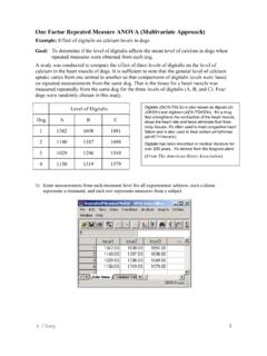
3 This assumption is known as the assumption of sphericity. The more accurate but complex explanation is as follows. Table 1 shows data from an experiment with three conditions. Imagine we calculated the differences between pairs of scores in all combinations of the treatment levels. Having done this, we calculated the variance of these differences. Sphericity is met when these variances are roughly equal. In these data there is some deviation from sphericity because the variance of the differences between conditions A and B ( ) is greater than the variance of the differences between A and C ( ) and between B and C ( ). However, these data have local circularity (or local sphericity) because two of the variances of differences are very similar. See Table 1: Hypothetical data to illustrate the calculation of the variance of the differences between conditions Condition A Condition B Condition C A B A C B C 10 12 8 2 2 4 15 15 12 0 3 3 25 30 20 5 5 10 35 30 28 5 7 2 30 27 20 3 10 7 Variance: What is the Effect of Violating the Assumption of Sphericity?

4 The effect of violating sphericity is a loss of power ( an increased probability of a Type II error) and a test statistic (F- ratio) that simply cannot be compared to tabulated values of the F- distribution (for more details see Field, 2009; 2013). Assessing the Severity of Departures from Sphericity Departures from sphericity can be measured in three ways: 1. Greenhouse and Geisser (1959) 2. Huynh and Feldt (1976) 3. The Lower Bound estimate (the lowest possible theoretical value for the data) Prof. Andy Field, 2012 Page 1 The Greenhouse- Geisser and Huynh- Feldt estimates can both range from the lower bound (the most severe departure from sphericity possible given the data) and 1 (no departure from sphjercitiy at all). For more detail on these estimates see Field (2013) or Girden (1992). SPSS also produces a test known as Mauchly's test, which tests the hypothesis that the variances of the differences between conditions are equal.

5 If Mauchly's test statistic is significant ( has a probability value less than .05) we conclude that there are significant differences between the variance of differences: the condition of sphericity has not been met. If, Mauchly's test statistic is nonsignificant ( p > .05) then it is reasonable to conclude that the variances of differences are not significantly different ( they are roughly equal). If Mauchly's test is significant then we cannot trust the F- ratios produced by SPSS. Remember that, as with any significance test, the power of Mauchley's test depends on the sample size. Therefore, it must be interpreted within the context of the sample size because: o In small samples large deviations from sphericity might be deemed non- . significant. o In large samples, small deviations from sphericity might be deemed significant.

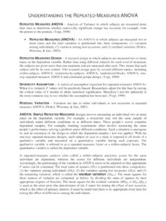
6 Correcting for Violations of Sphericity Fortunately, if data violate the sphericity assumption we simply adjust the defrees of freedom for the effect by multiplying it by one of the aforementioned sphericity estimates. This will make the degrees of freedom smaller; by reducing the degrees of freedom we make the F- ratio more conservative ( it has to be bigger to be deemed significant). SPSS applies these adjustments automatically. Which correction should I use? Look at the Greenhouse- Geisser estimate of sphericity ( ) in the SPSS handout. When > .75 then use the Huynh- Feldt correction. When < .75 then use the Greenhouse- Geisser correction. One-Way Repeated Measures ANOVA using SPSS. I'm a celebrity, get me out of here is a TV show in which celebrities (well, I mean, they're not really are they I'm struggling to know who anyone is in the series these days) in a pitiful attempt to salvage their careers (or just have careers in the first place) go and live in the jungle and subject themselves to ritual humiliation and/or creepy crawlies in places where creepy crawlies shouldn't go.

7 It's cruel, voyeuristic, gratuitous, car crash TV, and I love it. A particular favourite bit is the Bushtucker trials in which the celebrities willingly eat things like stick insects, Witchetty grubs, fish eyes, and kangaroo testicles/penises, nom nom noms . I've often wondered (perhaps a little too much) which of the bushtucker foods is most revolting. So I got 8 celebrities, and made them eat four different animals (the aforementioned stick insect, kangaroo testicle, fish eye and Witchetty grub) in counterbalanced order. On each occasion I measured the time it took the celebrity to retch, in seconds. The data are in Table 2. Prof. Andy Field, 2012 Page 2 Entering the Data The independent variable was the animal that was being eaten (stick, insect, kangaroo testicle, fish eye and witchetty grub) and the dependent variable was the time it took to retch, in seconds.

8 Levels of Repeated Measures variables go in different columns of the SPSS data editor. Therefore, separate columns should represent each level of a Repeated Measures variable. As such, there is no need for a coding variable (as with between- group designs). The data can, therefore, be entered as they are in Table 2. Save these data in a file called Table 2: Data for the Bushtucker example Celebrity Stick Insect Kangaroo Testicle Fish Eye Witchetty Grub 1 8 7 1 6 2 9 5 2 5 3 6 2 3 8 4 5 3 1 9 5 8 4 5 8 6 7 5 6 7 7 10 2 7 2 8 12 6 8 1 Draw an error bar chart of these data. The resulting graph is in Figure 1. Figure 1: Graph of the mean time to retch after eating each of the four animals (error bars show the 95% confidence interval) To conduct an ANOVA using a Repeated Measures design, activate the define factors dialog box by selecting.

9 In the Define Factors dialog box (Figure 2), you are asked to supply a name for the within- subject ( Repeated - Measures ) variable. In this case the Repeated Measures variable was the type of Prof. Andy Field, 2012 Page 3 animal eaten in the bushtucker trial, so replace the word factor1 with the word Animal. The name you give to the Repeated Measures variable cannot have spaces in it. When you have given the Repeated Measures factor a name, you have to tell the computer how many levels there were to that variable ( how many experimental conditions there were). In this case, there were 4 different animals eaten by each person, so we have to enter the number 4 into the box labelled Number of Levels. Click on to add this variable to the list of Repeated Measures variables. This variable will now appear in the white box at the bottom of the dialog box and appears as Animal(4).

10 If your design has several Repeated Measures variables then you can add more factors to the list (see Two Way ANOVA example below). When you have entered all of the Repeated Measures factors that were measured click on to go to the Main Dialog Box. Figure 2: Define Factors dialog box for Repeated Measures ANOVA Figure 3: Main dialog box for Repeated Measures ANOVA The main dialog box (Figure 3) has a space labelled within subjects variable list that contains a list of 4 question marks proceeded by a number. These question marks are for the variables representing the 4 levels of the independent variable. The variables corresponding to these levels should be selected and placed in the appropriate space. We have only 4 variables in the data editor, so it is possible to select all four variables at once (by clicking on the variable at the top, holding the mouse button down and dragging down over the other variables).