Transcription of Resonance and Impedance Matching
1 Chapter7 Resonance and Impedance MatchingMany common circuits make use of inductors and capacitors in different ways to achievetheir functionality. Filters, Impedance Matching circuits,resonators, and chokes are commonexamples. We study these circuits in detail and in particular weshall focus on the desirableproperties of the passive components in such ResonanceWe begin with the textbook discussion of Resonance ofRLCcircuits. These circuits aresimple enough to allow full analysis, and yet rich enough to formthe basis for most of thecircuits we will study in this simple second-order resonant circuit can also model a wide array of physicalphenomena, such as pendulums, mass-spring mechanical resonators,molecular Resonance ,microwave cavities, sections of transmission lines, and even large scale structures such asbridges. Understanding these circuits will afford a wide perspective into many shown in Fig. is deceptively simple. The impedanceseen by the sourceis simply given byZ=j L+1j C+R=R+j L 1 1 2LC ( )The Impedance is purely real at at theresonant frequencywhen (Z) = 0, or = 1 Resonance the Impedance takes on a minimal value.
2 It s worthwhile to investigate thecause of Resonance , or the cancellation of the reactive components due to the inductor and195196 chapter 7. Resonance AND Impedance MATCHINGZLRC+vs +vo Figure : A < 0 = 0vRvCvLvs > 0vRvCvLvsFigure : The phasor diagram of voltages in the seriesRLCcircuit (a) below Resonance ,(b) at Resonance , and (c) beyond Since the inductor and capacitor voltages are always 180 out of phase, and onereactance is dropping while the other is increasing, there isclearly always a frequency whenthe magnitudes are equal. Thus Resonance occurs when L=1 C. A phasor diagram, shownin Fig. , shows this in what s the magic about this circuit? The first observation isthat at Resonance , thevoltage across the reactances can be larger, in fact much larger, than the voltage across theresistorsR. In other words, this circuit has voltage gain. Of course it does not have powergain, for it is a passive circuit. The voltage across the inductor is given byvL=j 0Li=j 0 LvsZ(j 0)=j 0 LvsR=jQ vs( ) RESONANCE197where we have defined a circuitQfactor at Resonance asQ= 0LR( )It s easy to show that the same voltage multiplication occurs across the capacitorvC=1j 0Ci=1j 0 CvsZ(j 0)=1j 0 CvsR= jQ vs( )This voltage multiplication property is the key feature of the circuit that allows it to be usedas an Impedance s important to distinguish thisQfactor from the intrinsicQof the inductor andcapacitor.
3 For now, we assume the inductor and capacitor are ideal. We can re-write theQfactor in several equivalent forms owing to the equality of the reactances at resonanceQ= 0LR=1 0C1R= LCC1R=rLC1R=Z0R( )where we have defined theZ0=qLCas the characteristic Impedance of the Transfer FunctionLet s now examine the transfer function of the circuitH(j ) =vovs=Rj L+1j C+R( )H(j ) =j RC1 2LC+j RC( )Obviously, the circuit cannot conduct DC current, so there is azero in the transfer denominator is a quadratic polynomial. It s worthwhileto put it into a standard formthat quickly reveals important circuit parametersH(j ) =j RL1LC+ (j )2+j RL( )Using the definition ofQand 0for the circuitH(j ) =j 0Q 20+ (j )2+j 0Q( )Factoring the denominator with the assumption thatQ >12gives us the complex poles ofthe circuits = 02Q j 0r1 14Q2( )198 chapter 7. Resonance AND Impedance MATCHINGQ Q <12Q >12"""""""""""""""""""" """ !!!!!Figure : The root locus of the poles for a second-order transfer function as a function ofQ.
4 The poles begin on the real axis forQ <12and become complex, tracing a semi-circlefor poles have a constant magnitude equal to the resonant frequency|s|=vuut 204Q2,+ 20 1 14Q2,!= 0( )A root-locus plot of the poles as a function ofQappears in Fig. AsQ , the polesmove to the imaginary axis. In fact, the real part of the poles is inversely related to BandwidthAs shown in Fig. , when we plot the magnitude of the transfer function, we see that theselectivity of the circuit is also related inversely to theQfactor. In the limit thatQ ,the circuit is infinitely selective and only allows signals at Resonance 0to travel to the that the peak gain in the circuit is always unity, regardless ofQ, since at Resonance theLandCtogether disappear and effectively all the source voltage appears across the selectivity of the circuit lends itself well to filter applications (Sec. ). To charac-terize the peakiness, let s compute the frequency when the magnitude squared of the 1 00H(j 0) = 1 0 Figure : The transfer function of a seriesRLCcircuit.
5 The output voltage is taken atthe resistor terminals. IncreasingQleads to a more peaky drops by half|H(j )|2= 0Q 2( 20 2)2+ 0Q 2=12( )This happens when 20 2 0 /Q 2= 1( )Solving the above equation yields four solutions, corresponding to two positive and two neg-ative frequencies. The peakiness is characterized by the difference between these frequencies,or the bandwidth, given by = + = 0Q( )which shows that the normalized bandwidth is inversely proportional to the circuitQ 0=1Q( )You can also show that the Resonance frequency is the geometric mean frequency of the 3 dBfrequencies 0= + ( )200 chapter 7. Resonance AND Impedance MATCHINGLCRvs(t)vo(t)+Figure : A step function applied to a seriesRLCcircuit with output taken across Damping FactorSo far we have characterized the second order seriesRLCcircuit by its frequency response,leading to the concept of the resonant frequency 0and quality factorQ. An equivalentcharacterization involves the time domain response, particularly the step response of thecircuit.
6 This shall lead to the concept of the damping shown in Fig. , weshall now consider the output as the voltage across the capacitor. This corresponds to thecommon situation in digital circuits, where the load is a capacitive reactance of a let s recall the familiar step response of an RC circuit, orthe limit asL 0 in theseriesRLCcircuit, the circuit response to a step function is a rising exponential functionthat asymptotes towards the source voltage with a time scale = 1 the circuit has inductance, it s described by a second order differential KVL we can write an equation for the voltagevC(t)vs(t) =vC(t) +RCdvCdt+LCd2vCdt2( )with initial conditionsv0(t) =vC(t) = 0V( )andi(0) =iL(0) = 0A( )Fort >0, the source voltage switches toVdd. Thus Eq. has a constant source fort >0 Vdd=vC(t) +RCdvCdt+LCd2vCdt2( )In steady-state,ddt 0, leading toVdd=vC( )( ) RESONANCE201which implies that the entire voltage of the source appears across the capacitor, driving thecurrent in the circuit to zero.
7 Subtracting this steady-statevoltage from the solution, wecan simplify our differential equationvC(t) =Vdd+v(t)( )Vdd=Vdd+v(t) +RCdvdt+LCd2vdt2( )or more simply, the homogeneous equation0 =v(t) +RCdvdt+LCd2vdt2( )The solution of which is nothing but a complex exponentialv(t) =Aest, leading to thecharacteristic equation0 = 1 +RCs+LCs2= 1 + (s )2 + (s )2( )where we have defined =1 0( )and =12Q( )which has solutionss = p 2 1( )This equation can be characterized by the value , leading to the following three importantcases <1 Underdamped = 1 Critically Damped >1 Overdamped( )The terminology damped will become obvious we plot the generaltime-domain solution, we havevC(t) =Vdd+Aexp(s1t) +Bexp(s2t)( )which must satisfy the following boundary conditionsvC(0) =Vdd+A+B= 0( )andi(0) =CdvC(t)dt|t=0= 0( )202 chapter 7. Resonance AND Impedance =.3 =.5 = 1 = 2vC(t)Vddt Figure : The normalized step response of anRLCcircuit. The damping factor is variedto cover three important regions, an overdamped response with >1, a critically dampedresponse with = 1, and an underdamped response with < the following set of equationsAs1+Bs2= 0( )A+B= Vdd( )which has the following solutionA= Vdd1 ( )B= Vdd1 ( )where =s1s2.
8 So we have the following equationvC(t) =Vdd 1 11 es1t es2t ( )If the circuit is overdamped, >1, the poles are real and negatives=1 ( p 2 1) = s1s2<0( )The normalized response, with = 2,1, , , is shown in Fig. Qualitatively wesee that the = 2 circuit response resembles the familiar RC circuit. This is true (t)Vddt Figure : The step response of anRLCcircuit with low damping ( =.01). = 1, at which point the circuit is said to becritically damped. The circuit has two equalpoles ats=1 ( p 2 1) = 1 ( )In which case the time response is given bylim 1vC(t) =Vdd 1 e t/ t e t/ ( )As seen in Fig. , the circuit step response is faster with increasing 1, but still similarto the RC circuit. Theunderdampedcase, <1, is the most interesting case here, as theresponse is now markedly different. The circuitovershootsthe mark and settles down tothe steady-state value after oscillating. The amount of oscillation increases as the dampingfactor is reduced. The response with very low damping, =.
9 01 is shown in Fig. underdamped case is characterized by two complex conjugate poless = jp1 2=a jb( )Note the complex conjugate of theAcoefficient is simplyA = Vdd1 =Vdd 1 1= Vdd1 =B( )which allows us to write the voltage across the capacitor asvC(t) =Vdd+eat/ Aejbt +A e jbt ( )204 chapter 7. Resonance AND Impedance MATCHINGor more simplyvC(t) =Vdd+eat/ 2|A|cos( t+ )( )where|A|=Vdd|1 + |( )and = Vdd1 + ( )The oscillating frequency is determined by the imaginary part of the poles, =b/ = 0p1 2, which approaches the natural Resonance frequency as the damping is decay per period, or the envelope damping of the waveform, is determined bya, whichequals 0. This is why the damping factor controls the amount of overshoot and oscillationin the Storage inRLC Tank Let s compute the ebb and flow of the energy at Resonance . To begin, let s assume thatthere is negligible loss in the circuit. The energy across the inductor is given bywL=12Li2(t) =12LI2 Mcos2 0t( )Likewise, the energy stored in the capacitor is given bywC=12Cv2C(t) =12C 1 CZi( )d 2( )Performing the integral leads towC=12I2M 20 Csin2 0t( )The total energystoredin the circuit is the sum of these termsws=wL+wC=12I2M Lcos2 0t+1 20 Csin2 0t =12I2ML( )which is a constant!
10 This means that the reactive stored energyin the circuit does notchange and simply moves between capacitive energy and inductive energy. When the currentis maximum across the inductor, all the energy is in fact storedin the inductorwL,max=ws=12I2ML( ) RESONANCE205 YLRC isioFigure : A , the peak energy in the capacitor occurs when the current in the circuit drops tozerowC,max=ws=12V2MC( )Now let s re-introduce loss in the circuit. In each cycle, a resistorRwill dissipate energywd=P T=12I2MR 2 0( )The ratio of the energy stored to the energy dissipated is thuswswd=12LI2M12I2MR2 0= 0LR12 =Q2 ( )This gives us the physical interpretation of theQuality FactorQas 2 times the ratio ofenergy stored per cycle to energy dissipated per cycle in anRLCcircuitQ= 2 wswd( )We can now see that ifQ 1, then an initial energy in the tank tends to slosh back andforth for many cycles. In fact, we can see that in roughlyQcycles, the energy of the tankis parallelRLCcircuit shown in Fig. is the dual of the series circuit.