Transcription of Sensitivity, Background, Noise, and Calibration in Atomic ...
1 WHITEPAPERS ensitivity, background , noise , and Calibration in Atomic Spectroscopy: Effects on Accuracy and Detection LimitsIntroductionProper Calibration in Atomic spectroscopy and an understanding of uncertainty is fundamental to achieving accurate results. This paper provides a practical discussion of the effects of noise , error and concentration range of Calibration curves on the ability to determine the concentration of a given element with reasonable accuracy. The determination of lower limits of quantitation and lower limits of detection will also be accuracy is highly dependent on blank contamination, linearity of Calibration standards, curve-fitting choices and the range of concentrations chosen for Calibration .
2 Additional factors include the use of internal standards (and proper selection of internal standards) and instrumental settings. This paper is not intended to be a rigorous treatment of statistics in Calibration ; many references are available for this, such as Statistics in Analytical Chemistry1".The techniques of Atomic spectroscopy have been extensively developed and widely accepted in laboratories engaged in a broad range of elemental analyses, from ultra-trace quantitation at the sub-ppt level, to trace metal determination in the ppb to ppm range, to major component analysis at percent level fundamental part of analysis is establishing a Calibration curve for quantitative analysis. A series of known solutions is analyzed, including a blank prepared to contain no measurable amounts of the elements of interest.
3 This solution is designated as zero concentration and, together with one or more known standards, comprises the Calibration curve. Samples are then analyzed and compared to the mathematic calculation of signal vs. concentration established by the Calibration standards. Unfortunately, preparation of contamination-free blanks and diluents (especially when analyzing for many elements), perfectly accurate standards, and perfect laboratory measurements are all three most common Atomic spectroscopy techniques are Atomic absorption (AA) spectroscopy, ICP optical emission spectroscopy (ICP-OES) and ICP mass spectrometry (ICP-MS). Of these, ICP-OES and ICP-MS are very linear; that is, a plot of concentration vs. intensity forms a straight line over a wide range of concentrations (Figure 1).
4 AA is linear over a much smaller range and begins to curve downward at higher concentrations (Figure 2). Linear ranges are well understood, and, for AA, a rule of thumb can be applied to estimate the maximum working range using a non-linear paper will discuss the contributions of sensitivity , background , noise , Calibration range, Calibration mathematics and contamination on the ability to achieve best accuracy and lowest detection 1. Example of a linear Calibration curve in furnace AA, based on a more thorough and widely-ranging definition2. However, these procedures are specific to water, wastewater and other environmental are few widely accepted approaches for other matrices such as food, alloys, geological and plant materials, etc.
5 It is left to the lab doing the analysis to establish an approach to answer the question How low a concentration of a given element can we detect in a particular sample matrix? Because there exists a long history in most labs and many different techniques are employed ( , GC, LC, UV/Vis, FT-IR, AA, ICP, and many others) there are many opinions and approaches to this subject. How, Then, Do We Establish How Low We Can Go ?The simplest definition of a detection limit is the lowest concentration that can be differentiated from a blank. The blank should be free of analyte, at least to the limit of the technique used to measure it. Assuming the blank is clean , what is the lowest concentration that can be detected above the average blank signal?
6 One way to determine this is to first calibrate the instrument with a blank and some standards, calculate a Calibration curve, and then attempt to measure known solutions as samples at lower and lower concentrations until we reach the point that the reported concentration is indistinguishable from the blank. Unfortunately, no measurement at any concentration is perfect that is, there is always an uncertainty associated with every measurement in a lab. This is often called noise , and this uncertainty has several components. (A detailed discussion of sources of uncertainty is also a lengthy discussion3 and beyond the scope of this document.) So, to minimize uncertainty, it is common to perform replicate measurements and average challenge, then, is to find the lowest concentration that can be distinguished from the uncertainty of the blank.
7 This can be estimated by using a simple statistical approach. For example, EPA methods for water use such an approach. After Calibration , a blank is run as a sample 10 times, the 10 reported concentrations are averaged and the standard deviation is calculated. A test for statistical significance is applied (the Student s t-test) to calculate what the concentration would be that could be successfully differentiated from the blank with a high degree of confidence. In the EPA protocol, a 99% confidence is required. This equates to three times the standard deviation of 10 replicate readings. This is also known as a 3 (sigma) detection limit and is designated as the Instrument Detection Limit (IDL) for EPA is important to note that the statistically calculated detection limit is the lowest concentration that could even be detected in a simple, clean matrix such as 1% HNO3 it is not repeatable or reliable as a reported value in a real be more repeatable, the signal (with its associated uncertainty) must be significantly higher than the uncertainty of the blank, perhaps 5-10 times the standard deviation of the blank.
8 This is a judgment by the lab as to how confident the reported value should be. This concentration level might be called the lowest quantitation limit, sometimes known as PQL (practical quantitation limit), LOQ (limit of quantitation) or RL (reporting limit). There are no universally accepted rules for determining this Limits How Low Can We Go? Under ideal conditions, the detection limits of the various techniques range from sub part per trillion (ppt) to sub part per million (ppm), as shown in Figure 3. As seen in this figure, the best technique for an analysis will be largely dependent on the levels that need to measured, among other is important to realize that detection limits are not the same as reporting limits: just because a concentration can be detected does not mean it can be reported with confidence.
9 There are many factors associated with both detection limits and reporting limits which distinguish each, as will be seen in the following discussion of detection limits can be lengthy and is subject to many interpretations and assumptions there are even several definitions of detection limits . In Atomic spectroscopy, there are some commonly accepted approaches. Under some analytical protocols, the determination of detection limits is explicitly defined in a procedure, as in EPA methods and 6010 for ICP, and 6020 for ICP-MS, and for Figure 3 Figure 3. Detection limit ranges of the various Atomic spectroscopy Limit Ranges ( g/L)Figure 2. Example of a non-linear Calibration curve in , the EPA has guidelines in some methods for water samples that establish a lower reporting limit as a concentration that can be measured with no worse than +/- 30% accuracy in a prepared standard.
10 This rule is only applicable to the specific EPA method and in water labs apply the EPA detection limit methodologies simply because there are few commonly accepted and carefully defined approaches for other sample types. Some industries follow ASTM, AOAC or other industry guidelines, and some of these procedures include lower-limit analyzing a solid sample, the sample must first be brought into solution, which necessarily involves dilution. The estimation of detection or quantitation limits now needs to account for the dilution factor and matrix effects. For example, if 1 g of sample is dissolved and brought to a final volume of 100 mL, the detection limit in the solution must be multiplied by the dilution factor (100x in this example) to know what level of analyte in the original solid sample could have been measured if it could have been analyzed use the statistical estimate technique (3 detection limit), a clean matrix sample must be available, but this is not always possible.