Solving ODE in MATLAB - Texas A&M University

1 Solving ODE in MATLABP. HowardFall 2007 Contents1 Finding Explicit First order equations .. Second and Higher order equations .. Systems .. 32 Finding Numerical First- order equations with Inline Functions .. First order equations with M-files .. Systems of ODE .. Passing Parameters .. Second order equations .. 103 Laplace Transforms104 Boundary Value Problems115 Event Location126 Numerical Euler s Method .. Higher order Taylor Methods .. 187 Advanced ODE Stiff ODE .. 211 Finding Explicit SolutionsMATLAB has an extensive library of functions for Solving ordinary differential these notes, we will only consider the most First order EquationsThough MATLAB is primarily a numerics package, it can certainly solve straightforwarddifferential equations , for example, that we want to solve the firstorder differential equationy (x) =xy.

2 ( )We can use MATLAB s built-indsolve().The input and output for Solving this problem inMATLAB is given below.>>y = dsolve( Dy = y*x , x )y = C1*exp(1/2*x 2)Notice in particular that MATLAB uses capital D to indicate the derivative and requires thatthe entire equation appear in single quotes. MATLAB takestto be the independent variableby default, so herexmust be explicitly specified as the independent variable. Alternatively,if you are going to use the same equation a number of times, youmight choose to define itas a variable, say,eqn1.>>eqn1 = Dy = y*x eqn1 =Dy = y*x>>y = dsolve(eqn1, x )y = C1*exp(1/2*x 2)To solve an initial value problem, say, equation ( ) withy(1) = 1, use>>y = dsolve(eqn1, y(1)=1 , x )y =1/exp(1/2)*exp(1/2*x 2)or>>inits = y(1)=1 ;>>y = dsolve(eqn1,inits, x )y =1/exp(1/2)*exp(1/2*x 2)Now that we ve solved the ODE, suppose we want to plot the solution to get a rough idea ofits behavior.

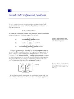
3 We run immediately into two minor difficulties:(1) our expression fory(x) isn tsuited for array operations (.*, ./, . ), and (2)y, as MATLAB returns it, is actually a symbol(asymbolic object). The first of these obstacles is straightforward to fix, usingvectorize().For the second, we employ the useful commandeval(),which evaluates or executes textstrings that constitute valid MATLAB commands. Hence, we can use1 Actually, whenever you do symbolic manipulations in MATLAB what you re really doing is >>x = linspace(0,1,20);>>z = eval(vectorize(y));>>plot(x,z)You may notice a subtle point here, thateval()evaluates strings (character arrays), andy,as we have defined it, is a symbolic object. However, vectorize converts symbolic objectsinto Second and Higher order EquationsSuppose we want to solve and plot the solution to the second order equationy (x) + 8y (x) + 2y(x) = cos(x);y(0) = 0, y (0) = 1.

4 ( )The following (more or less self-explanatory) MATLAB code suffices:>>eqn2 = D2y + 8*Dy + 2*y = cos(x) ;>>inits2 = y(0)=0, Dy(0)=1 ;>>y=dsolve(eqn2,inits2, x )y =1/65*cos(x)+8/65*sin(x)+(-1/130+53/1820 *14 (1/2))*exp((-4+14 (1/2))*x)-1/1820*(53+14 (1/2))*14 (1/2)*exp(-(4+14 (1/2))*x)>>z = eval(vectorize(y));>>plot(x,z) SystemsSuppose we want to solve and plot solutions to the system of three ordinary differentialequationsx (t) =x(t) + 2y(t) z(t)y (t) =x(t) +z(t)z (t) = 4x(t) 4y(t) + 5z(t).( )First, to find a general solution, we proceed as in Section , except with each equationnow braced in its own pair of (single) quotation marks:>>[x,y,z]=dsolve( Dx=x+2*y-z , Dy=x+z , Dz=4*x-4*y+5*z )x =2*C1*exp(2*t)-2*C1*exp(t)-C2*exp(3*t)+2 *C2*exp(2*t)-1/2*C3*exp(3*t)+1/2*C3*exp( t)y =2*C1*exp(t)-C1*exp(2*t)+C2*exp(3*t)-C2* exp(2*t)+1/2*C3*exp(3*t)-1/2*C3*exp(t)z =-4*C1*exp(2*t)+4*C1*exp(t)+4*C2*exp(3*t )-4*C2*exp(2*t)-C3*exp(t)+2*C3*exp(3*t)3 (If you use MATLAB to check your work, keep in mind that its choice of constants C1,C2, and C3 probably won t correspond with your own.)

5 For example, you might haveC= 2C1 + 1/2C3, so that the coefficients of exp(t) in the expression forxare , there is no such ambiguity when initial valuesare assigned.) Notice that sinceno independent variable was specified, MATLAB used its default,t. For an example in whichthe independent variable is specified, see Section Tosolve an initial value problem,we simply define a set of initial values and add them at the end of ourdsolve() we havex(0) = 1,y(0) = 2, andz(0) = 3. We have, then,>>inits= x(0)=1,y(0)=2,z(0)=3 ;>>[x,y,z]=dsolve( Dx=x+2*y-z , Dy=x+z , Dz=4*x-4*y+5*z ,inits)x =6*exp(2*t)-5/2*exp(t)-5/2*exp(3*t)y =5/2*exp(t)-3*exp(2*t)+5/2*exp(3*t)z =-12*exp(2*t)+5*exp(t)+10*exp(3*t)Finall y, plotting this solution can be accomplished as in Section >>t=linspace(0,.5,25);>>xx=eval(vectoriz e(x));>>yy=eval(vectorize(y));>>zz=eval( vectorize(z));>>plot(t, xx, t, yy, t, zz)The figure resulting from these commands is included as Figure : Solutions to equation ( ).

6 2 Finding Numerical SolutionsMATLAB has a number of tools for numerically Solving ordinary differential equations . Wewill focus on the main two, the built-in functionsode23andode45, which implement versionsof Runge Kutta 2nd/3rd- order and Runge Kutta 4th/5th- order , First- order equations with Inline FunctionsExample approximate the solution of the first order differential equationdydx=xy2+y;y(0) = 1,on the intervalx [0, .5].For any differential equation in the formy =f(x, y), we begin by defining the functionf(x, y). For single equations , we can definef(x, y) as an inline function. Here,>>f=inline( x*y 2+y )f =Inline function:f(x,y) = x*y 2+yThe basic usage for MATLAB s solverode45isode45(function,domain,initi al condition).That is, we use>>[x,y]=ode45(f,[0 .5],1)and MATLAB returns two column vectors, the first with values ofxand the second withvalues ofy.

7 (The MATLAB output is fairly long, so I ve omitted it here.)Sincexandyarevectors with corresponding components, we can plot the values with>>plot(x,y)which creates Figure the approximating this solution, the algorithmode45hasselected a certain partition of the interval [0, .5], and MATLAB has returned a value ofyateach point in this partition. It is often the case in practicethat we would like to specify thepartition of values on which MATLAB returns an approximation. For example, we mightonly want to approximatey(.1),y(.2), ..,y(.5). We can specify this by entering the vectorof values [0, .1, .2, .3, .4, .5] as the domain inode45. That is, we use>>xvalues=0:.1:.5xvalues =0 >>[x,y]=ode45(f,xvalues,1)x = : Plot of the solution toy =xy2+y, withy(0) = = is important to point out here that MATLAB continues to useroughly the same partitionof values that it originally chose; the only thing that has changed is the values at which it isprinting a solution.

8 In this way, no accuracy is options are available for MATLAB sode45solver, giving the user lim-ited control over the algorithm. Two important options are relative and absolute tolerance,respecivelyRelTolandAbsTolin MATLAB . At each step of theode45algorithm, an erroris approximated for that step. Ifykis the approximation ofy(xk) at stepk, andekis theapproximate error at this step, then MATLAB chooses its partition to insureek max(RelTol yk,AbsTol),where the default values are RelTol = .001 and AbsTol = .000001. As an example for whenwe might want to change these values, observe that ifykbecomes large, then the errorekwill be allowed to grow quite large. In this case, we increasethe value of RelTol. For theequationy =xy2+y, withy(0) = 1, the values ofyget quite large asxnears 1. In fact,with the default error tolerances, we find that the command>>[x,y]=ode45(f,[0,1],1);6leads to an error message, caused by the fact that the values ofyare getting too large asxnears 1.

9 (Note at the top of the column vector forythat it is multipled by 1014.) In orderto fix this problem, we choose a smaller value for RelTol.>>options=odeset( RelTol ,1e-10);>>[x,y]=ode45(f,[0,1],1,options) ;>>max(y)ans = +07In addition to employing the option command, I ve computed the maximum value ofy(x)to show that it is indeed quite large, though not as large as suggested by the previouscalculation. First order equations with M-filesAlternatively, we can solve the same ODE as in Example by first definingf(x, y) as yprime = firstode(x,y);% FIRSTODE: Computes yprime = x*y 2+yyprime = x*y 2 + y;In this case, we only require one change in theode45command: we must use a pointer @to indicate the M-file. That is, we use the following commands.>>xspan = [0,.5];>>y0 = Systems of ODES olving a system of ODE in MATLAB is quite similar to Solving asingle equation, thoughsince a system of equations cannot be defined as an inline function we must define it as the system of Lorenz equations ,2dxdt= x+ ydydt= x y xzdzdt= z+xy,( )2 The Lorenz equations have some properties of equations arising in atmospherics.

10 Solutions of the Lorenzequations have long served as an example for chaotic for the purposes of this example, we will take = 10, = 8/3, and = 28, as well asx(0) = 8,y(0) = 8, andz(0) = 27. The MATLAB M-file containing the Lorenz equationsappears xprime = lorenz(t,x);%LORENZ: Computes the derivatives involved in Solving the%Lorenz ;beta=8/3;rho=28;xprime=[-sig*x(1) + sig*x(2); rho*x(1) - x(2) - x(1)*x(3);-beta*x(3) + x(1)*x(2)];Observe thatxis stored as x(1),yis stored as x(2), andzas stored as x(3). Additionally,xprimeis a column vector, as is evident from the semicolon following the first appearance ofx(2). If in the Command Window, we type>>x0=[-8 8 27];>>tspan=[0,20];>>[t,x]=ode45(@lorenz ,tspan,x0)Though not given here, the output for this last command consists of a column of timesfollowed by a matrix with three columns, the first of which corresponds with values ofxat the associated times, and similarly for the second and third columns foryandz.