Transcription of Two-Way Independent ANOVA - Discovering Statistics
1 Two-Way Independent ANOVA Using SPSS. Introduction Up to now we have looked only at situations in which a single Independent variable was manipulated. Now we move onto more complex designs in which more than one Independent variable has been manipulated. These designs are called Factorial Designs. When you have two Independent variables the corresponding ANOVA is known as a Two-Way ANOVA , and when both variables have been manipulated using different participants the test is called a Two-Way Independent ANOVA (some books use the word unrelated rather than Independent ). So, a Two-Way Independent ANOVA . is used when two Independent variables have been manipulated using different participants in all conditions. The Beer-Goggles' Effect A psychologist was interested in the effects of alcohol on mate selection at night-clubs. Her rationale was that after alcohol had been consumed, subjective perceptions of physical attractiveness would become more inaccurate (the well- known beer-goggles effect').
2 She was also interested in whether this effect was different for men and women. She picked 48 students: 24 male and 24 female. She then took groups of 8 participants to a night-club and gave them no alcohol (participants received placebo drinks of alcohol-free lager), 2 pints of strong lager, or 4 pints of strong lager. At the end of the evening she took a photograph of the person that the participant was chatting up. She then got a pool of Independent raters to assess the attractiveness of the person in each photograph (out of 100). The data are presented in Table 1. Table 1: Data for the beer-goggles effect Alcohol None 2 Pints 4 Pints Gender Female Male Female Male Female Male 65 50 70 45 55 30. 70 55 65 60 65 30. 60 80 60 85 70 30. 60 65 70 65 55 55. 60 70 65 70 55 35. 55 75 60 70 60 20. 60 75 60 80 50 45. 55 65 50 60 50 40. We saw earlier in the module that one-way ANOVA could be conceptualized as a regression equation (a general linear model) see Field (2013), Chapter 11 for more detail.
3 We'll now consider how we extend this linear model to incorporate two Independent variables. To keep things as simple as possible I want you to imagine that we have only two levels of the alcohol variable in our example (none and 4 pints). As such, we have two predictor variables, each with two levels. All of the general linear models we've considered take the general form of: outcome' = model + error'. For example, when we encountered multiple regression in we saw that this model was written as: ' = / + 0 0' + 2 2' + + 4 4' + '. Also, when we came across one-way ANOVA , we adapted this regression model to conceptualize our Viagra example, as: Prof. Andy Field, 2016 Page 1. Libido' = / + 2 high' + 0 low' + '. In this model, the High and Low variables were dummy variables ( , variables that can take only values of 0 or 1). In our current example, we have two variables: gender (male or female) and alcohol (none and 4 pints).
4 We can code each of these with zeros and ones, for example, we could code gender as male = 0, female = 1, and we could code the alcohol variable as 0 = none, 1 = 4 pints. We could then directly copy the model we had in one-way ANOVA : Attractiveness' = / + 0 Gender' + 2 Alcohol' + '. However, this model does not consider the interaction between gender and alcohol. If we want to include this term too, then the model simply extends to become (first expressed generally and then in terms of this specific example): Attractiveness' = / + 0 A ' + 2 B' + = AB' + '. Attractiveness' = / + 0 Gender' + 2 Alcohol' + = Interaction' + '. The question is: how do we code the interaction term? The interaction term represents the combined effect of alcohol and gender; to get any interaction term you simply multiply the variables involved. This is why you see interaction terms written as gender alcohol, because in regression terms the interaction variable literally is the two variables multiplied by each other.
5 For more detail about how all of the coding works read Field (2013), Chapters 10 and 12. For the purpose of this exercise all I really want you to understand is that (1) we're still fitting a linear model; (2) SPSS will code your predictors ( Independent variables) using the dummy coding that we have discussed before; and (3) we include an interaction term, which is coded by multiplying the dummy codes for any of the predictors involved in the interaction. Two-Way Independent ANOVA Using SPSS. Inputting Data Levels of between group variables go in a single column of the SPSS data editor. Applying the rule above to the data we have here we are going to need to create 2 different coding variables (seeField, 2013, Chapter 3) in the data editor. These columns will represent gender and alcohol consumption. So, create a variable called Gender in the data editor and activate the labels dialog box. You should define value labels to represent the two genders.
6 We have had a lot of experience with coding values, so you should be fairly happy about assigning numerical codes to different groups. I recommend using the code Male = 0, and Female = 1. Once you have done this, you can enter a code of zero or one in this column indicating to which group the participant belonged. Create a second variable called Alcohol and assign group codes by using the labels dialog box. I suggest that you code this variable with three values: Placebo (no Alcohol) = 1, 2 Pints = 2, and 4 pints = 3. You can now enter 1, 2 or 3 into this column to represent the amount of alcohol consumed by the participant. Remember that if you turn the value labels option on ( ) you will see text in the data editor rather than the numerical codes. Now, the way this coding works is as follows: Gender Alcohol Participant was .. 0 1 Male who consumed no alcohol 0 2 Male who consumed 2 pints 0 3 Male who consumed 4 pints 1 1 Female who consumed no alcohol 1 2 Female who consumed 2 pints 1 3 Female who consumed 4 pints Once you have created the two coding variables, you can create a third variable in which to place the values of the dependent variable.
7 Call this variable attract and use the labels option to give it the fuller name of Attractiveness of Date'. In this example, there are two Independent variables and different participants were used in each condition: Prof. Andy Field, 2016 Page 2. hence, we can use the general factorial ANOVA procedure in SPSS. This procedure is designed for analysing between- group factorial designs. Enter the data into SPSS. Save the data onto a disk in a file called Plot an error bar graph of the mean attractiveness of mates across the different levels of alcohol. Plot an error bar graph of the mean attractiveness of mates selected by males and females. The Main Dialog Box To access the main dialog box use the file path . The resulting dialog box is shown in Figure 1. First, select the dependent variable Attractiveness from the variables list on the left-hand side of the dialog box and drag it to the space labelled Dependent Variable or click on.
8 In the space labelled Fixed Factor(s) we need to place any Independent variables relevant to the analysis. Select Alcohol and Gender in the variables list (these variables can be selected simultaneously by holding down Ctrl while clicking on the variables) and drag them to the Fixed Factor(s) box (or click on ). There are various options available to us, we only need worry about the ones covered in this handout (anyone interested in further options should read my 2013 textbook, chapter 13). Figure 1: Main dialog box for univariate ANOVA . Simple and horrible looking graphs of Interactions Click on to access the dialog box in Figure 2. The plots dialog box allows you to select line graphs of your data and these graphs are very useful for interpreting interaction effects (however, really we should plot graphs of the means before the data are analysed). We have only two Independent variables, and the most useful plot is one that shows the interaction between these variables (the plot that displays levels of one Independent variable against the other).
9 In this case, the interaction graph will help us to interpret the combined effect of gender and alcohol consumption. Select Alcohol from the variables list on the left-hand side of the dialog box and drag it to the space labelled Horizontal Axis (or click on ). In the space labelled Separate Lines place the remaining Independent variable, Gender. It doesn't matter which way round the variables are plotted; you should use your discretion as to which way produces the most sensible graph. When you have moved the two Independent variables to the appropriate box, click on and this plot will be added to the list at the bottom of the box. You can plot a whole variety of graphs, and if you had a third Independent variable, you have the option of plotting different graphs for each level of that third variable by specifying a variable under the heading Separate Plots. When you have finished specifying graphs, click on to return to the main dialog box.
10 Prof. Andy Field, 2016 Page 3. Figure 2: Specifying plots Post Hoc Tests The post hoc tests dialog box is obtained by clicking on in the main dialog box (Figure 3). The variable Gender has only two levels and so we don't need to select post hoc tests for that variable (because any significant effects can reflect only the difference between males and females). However, there were three levels of the Alcohol variable (no alcohol, 2 pints and 4 pints); hence we can conduct post hoc tests (although remember that normally you would conduct contrasts or post hoc tests, not both). First, you should select the variable Alcohol from the box labelled Factors and transfer it to the box labelled Post Hoc Tests for. My recommendations for which post hoc procedures to use are in last weeks handout (and I don't want to repeat myself). Suffice to say you should select the ones in Figure 3! Click on to return to the main dialog box.