Transcription of Understanding Time Current Curves - Maverick Technologies
1 WHITE PAPER Understanding time Current Curves . Understanding time Current Curves David Paul , Engineering Design Manager, Maverick Technologies A time Current curve (TCC) plots the The orange curve is the transformer damage curve. The green Curves are the cable damage Curves . Each one interrupting time of an overcurrent of these items will be explained. The system represented device based on a given Current level. by this curve is well coordinated and adequately protected These Curves are provided by the from damage. It also has minimal Arc Flash hazard category ratings due to low instantaneous circuit breaker trip values. manufacturers of electrical overcurrent interrupting devices such as fuses and The One Line Diagram and TCC curve show a typical hypothetical circuit breakers.
2 These Curves are part industrial power system (Figure 2). There is a utility delivery of the product acceptance testing point with power supplied at a medium voltage level (In this case 4160 volts), which feeds the primary side of a power required by Underwriters Laboratories transformer through a medium voltage fused switch containing (UL) and other rating agencies. an E class fuse. The 480 volt secondary side of the transformer feeds a piece of low voltage power switchgear utilizing draw The shape of the Curves is dictated by both the physical out low voltage power circuit breakers for the main and feeder construction of the device as well as the settings selected circuit breakers.
3 The TCC plot also displays the transformer in the case of adjustable circuit breakers. The time and cable damage Curves . These Curves are based on Current Curves of a device are important for engineers to accepted industry consensus standards published by understand because they show graphically the response ANSI (for the transformer) and ICEA (for the cables). of the device to various levels of overcurrent. The Curves allow the power system engineer to graphically represent the selective coordination of overcurrent devices in an electrical system. Modern power system design software packages such as EasyPower, SKM Power Tools, and Etap contain graphical libraries of Curves to allow the power system engineer the ability to plot, analyze and print the Curves with minimal effort compared to the previous methods used when coordinating a power system.
4 TCC Item Identification The TCC Curves shown (Figure 1) plot the interrupting response time of a Current interrupting device versus time . Current is shown on the horizontal axis using a logarithmic scale and is plotted as amps X 10X. time is shown on the vertical axis using a logarithmic scale and is plotted in seconds X 10X. The light blue curve is a switchgear feeder circuit breaker curve. The violet curve is the switchgear main circuit breaker curve. Figure 1: Typical time Current Curve Plot The red curve is the transformer primary fuse curve. 1/6. WHITE PAPER Understanding time Current Curves . Interpreting the damage Curves is fairly straightforward. Operating conditions (overcurrent protection) must be kept to the left of the damage curve to guarantee no permanent damage is done to the transformer or cable in question (Figure 3).
5 Operating conditions which allow operation to the right of the damage curve subject the device in question to currents that cause permanent irreversible damage, a shortened lifespan and possible catastrophic failure. Therefore the overcurrent and circuit breaker coordination schemes must take this into account during the initial design phase. There are two transformer damage Curves (shown in orange), one is dashed and the other is solid. The solid damage curve is the unbalanced damage curve which takes into account a derating factor for transformer winding type and fault type. The dashed damage curve is the 100% rating curve with no derating consideration. The transformer inrush Current is also plotted as a single point on the TCC diagram.
6 Again, as part of the initial design, the transformer inrush Current must be to the left of the transformer primary fuse curve otherwise the fuse will open when the transformer is energized. Figure 2: The One Line Diagram shown These differences in the unbalanced and 100% damage Curves can in figure 2 is represented in the TCC be mitigated with additional protective relaying to allow the 100%. Curve in figure 3 curve to be used for power system design without the risk of transformer damage. There are three cable damage Curves (shown in green). There is one curve for each cable represented on the one line diagram. As part of the initial design, the overcurrent interrupting device must limit the fault Current to the left of the damage curve to prevent permanent damage.
7 The damage Curves for the cables are dependent on size, insulation type and raceway configuration. The light blue curve represents the circuit breaker settings for the feeder circuit breaker. The lower portion of the curve (below .05 seconds or 3. cycles on the time axis) is the instantaneous trip function. The purpose of the instantaneous trip is to trip the circuit breaker quickly with no intentional delay (no more than a few cycles) on high magnitude fault currents. This quick trip protects electrical distribution equipment from damage and keeps arc flash hazard categories low. Clearly these type faults must be interrupted quickly and do not allow the system to wait and see if the fault will self clear.
8 The minimum instantaneous setting determines the minimum trip setting for the circuit breaker. In the case shown above, the instantaneous setting is 2400 amps and the Figure 3: Selectively coordinated maximum value displayed is available fault Current at the circuit breaker. electrical power system. Major elements Small changes in the instantaneous setting can result in significant of the time Current curve are labeled. changes in the Arc Flash Hazard category, so this is a setting which must be carefully selected according to sound engineering principles. 2/6. WHITE PAPER Understanding time Current Curves . The next section of the curve moving up the time axis is determined by the short time settings.
9 Short time settings cover the time range from to seconds (3 to 30 cycles). The purpose of short time settings is to allow a time - based delay to elapse before tripping the circuit breaker for moderate Current faults. This allows moderate faults time to clear themselves without tripping the circuit breaker. Examples of these types of overcurrents would be the inrush on a large motor starting or a transformer inrush when it is first energized. The short time pickup setting shifts the curve on the Current axis. Increasing the short time pickup settings shifts the curve to the right and conversely lower settings shift the curve to the left. The short time delay setting moves the knee of the curve vertically on the time axis.
10 Increasing the short time delay setting moves the knee vertically up the time axis. Similarly, decreasing the settings moved the knee lower on the vertical axis. The described curve shifts are depicted on the TCC plots below. (Figures 4 - 7). Figure 4: Short time Base Case Figure 5: Decreased Short time Pickup STPU= ST DLY=Min Notice curve shift to left STPU= Figure 6: Increased Short time Pickup Figure 7: Increased Short time delay Notice curve shift to Right STPU=4 Notice curve shift vertically ST DLY=Max 3/6. WHITE PAPER Understanding time Current Curves . The next section of the curve moving up the time axis is the long time section. Long time settings cover the time range from to 1000 seconds.