Lecture 7 Static Structural Analysis

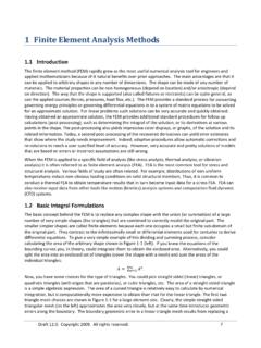
1 Finite Element Analysis Methods - Rice University

1 Finite Element Analysis Methods ... it is often referred to as finite element analysis (FEA). FEA is the most common tool for stress and structural ...

  Analysis, Methods, Elements, Finite, Element analysis, 1 finite element analysis methods

Lecture 1 Introduction to ANSYS Workbench - Rice …

This training course covers the basics of using ANSYS Mechanical in performing structural and thermal analyses. It is intended for all new or occasional ANSYS Mechanical users, regardless

  Lecture, Introduction, Basics, Ansys, Workbench, Lecture 1 introduction to ansys workbench

Types of Control: Open loop, feedback, feedforward

Feedback Control “Understand Your Technical World” ... • or better, why do you need a control system at all? • consider ovens, A/C units, airplanes, manufacturing, pumping stations, etc ... Design of dynamics through feedback Allows the dynamics (behavior) of the system to be modified ...

  System, Design, Control, Feedback, Control system, Feedback control

Lecture 9 Thermal Analysis - Rice University

thermal resistance. q TCC T target T contact The amount of heat flow across a contact interface is defined by the contact heat flux expression ^q” shown here: • T contact is the temperature of the contact surface and • T target is the temperature of the target surface. … Thermal ontact

  Lecture, Analysis, Thermal, Interface, Lecture 9 thermal analysis

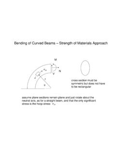
curved beam strength - Rice University

kr σθθ=− − + = r r ... iar r m ari y r i r iar m yri ari ayri ar r m yrai r

Introduction to ANSYS Mechanical

– The “2D” switch must be set on the Project page prior to importing geometry. •Each node in a 2D element has two translational degrees of freedom (UX and UY) for structural or one temperature DOF for thermal. •2D solids are used to represent three types of 3D geometry, “Axisymmetric”, “Plane stress” and “Plane strain”.

  Introduction, Mechanical, Geometry, Ansys, Introduction to ansys mechanical

8 Flat Plate Analysis - Rice University

Then, the plots are pretty, but wrong. If the edges of the plate are simply sitting on top of to walls, then the wall could not pull down on the corner. ... reaction forces appear, then move the split line away from the corner and repeat the process. It may be a slow procedure, but it can lead you to the correct lift off regions. ...

  Analysis, Plate, Split, Flat, Plot, 8 flat plate analysis

12 Buckling Analysis - Rice University

those terms even though finite element analysis lets you conduct buckling studies in 1D, 2D, and 3D. For a material, stiffness refers to either its elastic modulus, E, or to its shear modulus, G = E / (2 + 2 v) where v is Poisson’s ratio.

  Analysis, Elements, Finite, Finite element analysis

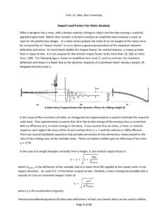
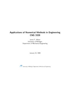
Impact Load Factors - Rice University

Maximum horizontal stress (143 MPa) is at the center plane top and bottom Of course, since the static model is linear there is no need to re-run the model (unless you want pretty plots). The static maximum fiber stress (SX) of 26.0 MPa could be multiplied by the 5.48 vertical Impact Factor to find the dynamic maximum SX stress of 143 MPa.

  Factors, Impact, Load, Stress, Impact load factors

Space Truss and Space Frame Analysis - Rice University

space frame is a combination of individual beam‐column elements that resists loadings by a combination of bending, axial member forces, and transverse (shear) forces, and axial torsion. Therefore, it is a more efficient

  Frame, Space, Space frame

Applications of Numerical Methods in Engineering CNS 3320

Linear Systems Example: Circuit Analysis Kirchhoff’s Laws: 1. The sum of all voltage changes around any closed loop is zero: Xne i=1 ∆V i = 0 2. The sum of all currents at any node is zero. Xnb i=1 ∆I i = 0 Application of these two laws to an electrical circuit facilitates the formulation of a system of n linear equations when n unknown ...

  Linear

29 CONNECTION DESIGN – DESIGN REQUIREMENTS

• Connectors behave in a linear-elastic manner until failure. • Connectors have unlimited ductility. However, in reality, connected parts such as end plates, angles etc. are flexible and deform even at low load levels. Further, their behaviour is highly non-linear due to slip, lack of fit, material non-linearity and residual stresses.

  Linear, Design, Requirements, Connection, Elastic, Connection design design requirements

Vibration, Normal Modes, Natural Frequencies, Instability

problem, the linear dependence of the force on x may be an approximation for small x.) In order to get a solution, the initial displacement and initial velocity must be specified. Common formulations are: x(0) = 0, and dx dt (0) = V 0 (The mass dxresponds to an initial impulse.); or x(0) = X 0 and dt (0) = 0 (The mass is given an initial ...

  Linear

VEHICLE DYNAMICS PROJECT - IIT Hyderabad

•VEHICLE SUSPENSION OPTIMIZATION FOR STOCHASTIC INPUTS, KAILAS VIJAY INAMDAR • On the Control Aspects of Semiactive Suspensions for Automobile Applications, Emmanuel D. Blanchard • Analysis design of VSS using Matlab simulink, Ali Md. Zadeh • MR damper and its application for semi-active control of vehicle suspension system , G.Z. Yao, …

  Project, Vehicle, Dynamics, Vehicle dynamics project

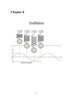
Chapter8 Oscillations

AP Physics Multiple Choice Practice – Oscillations 1. A mass m, attached to a horizontal massless spring with spring constant k, is set into simple harmonic motion. Its maximum displacement from its equilibrium position is A. What is the mass’s speed as it passes through its equilibrium position? (A)A k m (B)A m k (C) 1 A k m (D) 1 A m k 2.

  Multiple

A Beginner’s Guide

modulus when viewed on a log scale against a linear temperature scale, shown in Figure 5. A concurrent peak in the tan delta is also seen. The value reported as the Tg varies with industry with the onset of the E’ drop, the peak of the tan delta, and the peak of the E’ curve being the most commonly used. Figure 4.

  Guide, Linear, Beginner, A beginner s guide