
Plotting in Scilab - Openeering
Plotting in Scilab www.openeering.com page 3/17 Step 1: Basic plot with LaTex annotations Here, we plot the function: U L 1 1 6 on the interval > F5,5. // Close all opened figures and clear workspace
Download Plotting in Scilab - Openeering

Information
Domain:
Source:
Link to this page:
Documents from same domain

NUMERICAL ANALYSIS USING SCILAB SOLVING …
www.openeering.comNonlinear equations www.openeering.com page 1/25 NUMERICAL ANALYSIS USING SCILAB: SOLVING NONLINEAR EQUATIONS In this tutorial we provide a collection of numerical methods for solving nonlinear

NUMERICAL SIMULATION OF AN ORGANIC …
www.openeering.comOrganic_Rankine_Cycle www.openeering.com page 2/14 1. Introduction In this article, we present a numerical solver for the simulation of an Organic Rankine Cycle (ORC)

MODELING IN XCOS USING MODELICA - Openeering
www.openeering.comwww.openeering.com powered b y MODELING IN XCOS USING MODELICA In this tutorial we show how to model a physical system described by ODE using the Modelica extensions of the Xcos environment.

HOW TO DEVELOP A GRAPHICAL SER NTERFACE …
www.openeering.comwww.openeering.com powered by HOW TO DEVELOP A GRAPHICAL USER INTERFACE (GUI) IN SCILAB. In this tutorial we show how to create a GUI in Scilab for an ODE problem. The adopted problem is the LHY model already used in other tutorials.

powered by INTRODUCTION TO CONTROL …
www.openeering.comwww.openeering.com powered by INTRODUCTION TO CONTROL SYSTEMS IN SCILAB In this Scilab tutorial, we introduce readers to the Control System Toolbox that is available in Scilab/Xcos and known as CACSD.

MODELING IN XCOS USING MODELICA - Openeering
www.openeering.comwww.openeering.com powered b y MODELING IN XCOS USING MODELICA In this tutorial we show how to model a physical system described by ODE using the Modelica extensions of the Xcos environment.

powered by MULTIOBJECTIVE OPTIMIZATION AND …
www.openeering.comwww.openeering.com powered by MULTIOBJECTIVE OPTIMIZATION AND GENETIC ALGORITHMS In this Scilab tutorial we discuss about the importance of multiobjective optimization and we give an overview of all possible Pareto frontiers.

NUMERICAL ANALYSIS USING SCILAB ERROR ANALYSIS …
www.openeering.comError analysis and propagation www.openeering.com page 4/10 Step 5: Cancellation error It is interesting to analyze the arithmetic operations when we consider
Related documents
Basic Graphics in R - Harvard University
bcb.dfci.harvard.eduPlot of data.frame elements If the rst argument to plot() is a data.frame, this can be as simply as plot(x,y) providing 2 columns (variables in the data.frame). Lets look at the data in the data.frame airquality which measured the 6 air quality in New
LabVIEW Lesson 6 – File I/O and Plotting
boson.physics.sc.eduLabVIEW Lesson 6 – File I/O and Plotting Lesson Overview • Why use file I/O? ... File I/O formats depend on the type of files being used. 3 types of formats exist: text, binary, and datalog. ... the plot lines, the type of data points (useful when plotting multiple sets of data), and many other options. ...
Using SAS’s PROC GPLOT to plot data and lines
cob.jmu.eduUsing SAS’s PROC GPLOT to plot data and lines PROC GPLOT creates “publication quality” color graphics which can easily be exported into documents, presentations, etc. To export the graphs for future use click on file, export. In the dialog box choose a
Basic Plotting with Python and Matplotlib
courses.csail.mit.eduThe basic syntax for creating line plots is plt.plot(x,y), where x and y are arrays of the same length that specify the (x;y) pairs that form the line. For example, let’s plot the cosine function from 2 to 1.
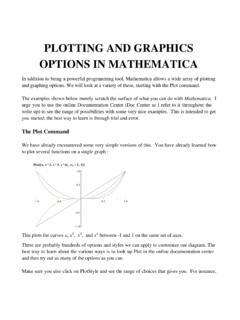
PLOTTING AND GRAPHICS OPTIONS IN MATHEMATICA
dslavsk.sites.luc.eduPLOTTING AND GRAPHICS OPTIONS IN MATHEMATICA In addition to being a powerful programming tool, Mathematica allows a wide array of plotting and graphing options. We will look at a variety of these, starting with the Plot command. ... Plot x, x^2, x^3, x ...

Unit 9 Describing Relationships in Scatter Plots and Line ...
lycofs01.lycoming.edu56 Unit 9 Describing Relationships in Scatter Plots and Line Graphs Objectives: • To construct and interpret a scatter plot or line graph for two quantitative variables
Math 141 - Quantile-Quantile Plots
people.reed.eduThe QQ plot The quantile–quantile plot, or QQplot, is a simple graphical method for comparing two sets of sample quantiles. Plot the pairs of order statistics (X (k);Y (k)): If the two datasets come from the same distribution, the points ... Math 141 - Quantile-Quantile Plots ...
Plotting functions of more than one variable with Mathematica
physics.weber.eduPlotting functions of more than one variable with Mathematica Physics 3510, Weber State University This tutorial assumes that you are already somewhat familiar with Mathematica.
Split Plots - Statistics
users.stat.umn.eduAll split plots in the same whole plot get the same level of the whole plot treatment factor. All levels of the split plot treatment factor occur in each whole plot. The restricted randomization is equivalent to the two randomizations of the unit structure approach.
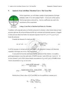
9. Analysis of an Acid-Base Titration Curve: The Gran Plot
web.mnstate.eduThe Gran plot in the acidic region gives accurate results even if there is CO2 dissolved in the strong base titrant. The Gran plot in the basic region can be used to measure CO2 in the strong base. For completeness, we note that if weak base, B, is titrated with a strong acid, the Gran
Related search queries
Basic Graphics in R, Plot, Lesson 6, File I/O, The Plot, Using SAS’s PROC GPLOT to plot data, Basic Plotting with Python and Matplotlib, PLOTTING AND GRAPHICS OPTIONS IN, Describing Relationships in Scatter Plots, Math 141 - Quantile-Quantile Plots, Plotting functions of more than one variable with Mathematica, Split plots, Gran plot