The Multivariate Gaussian Distribution

1 The Multivariate Gaussian DistributionChuong B. DoOctober 10, 2008A vector-valued random variableX= X1 Xn Tis said to have amultivariatenormal (or Gaussian ) distributionwith mean Rnand covariance matrix Sn++1if its probability density function2is given byp(x; , ) =1(2 )n/2| |1/2exp 12(x )T 1(x ) .We write this asX N( , ). In these notes, we describe Multivariate Gaussians and someof their basic Relationship to univariate GaussiansRecall that the density function of aunivariate normal (or Gaussian ) distributionisgiven byp(x; , 2) =1 2 exp 12 2(x )2 .Here, the argument of the exponential function, 12 2(x )2, is a quadratic function of thevariablex.

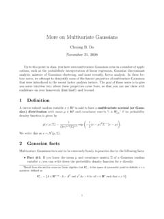
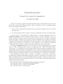
2 Furthermore, the parabola points downwards, as the coefficient of the quadraticterm is negative. The coefficient in front,1 2 , is a constant that does not depend onx;hence, we can think of it as simply a normalization factor used to ensure that1 2 Z exp 12 2(x )2 = from the section notes on linear algebra thatSn++is the space of symmetric positive definiten nmatrices, defined asSn++= A Rn n:A=ATandxTAx >0 for allx Rnsuch thatx6= 0 .2In these notes, we use the notationp( ) to denote density functions, instead offX( ) (as in the sectionnotes on probability theory). 10 50510 10 1: The figure on the left shows a univariate Gaussian density for a single figure on the right shows a Multivariate Gaussian density overtwo the case of the Multivariate Gaussian density, the argument ofthe exponential function, 12(x )T 1(x ), is aquadratic formin the vector variablex.

3 Since is positivedefinite, and since the inverse of any positive definite matrix isalso positive definite, thenfor any non-zero vectorz,zT 1z >0. This implies that for any vectorx6= ,(x )T 1(x )>0 12(x )T 1(x )< in the univariate case, you can think of the argument of the exponential function asbeing a downward opening quadratic bowl. The coefficient in front ( ,1(2 )n/2| |1/2) has aneven more complicated form than in the univariate case. However, it still does not dependonx, and hence it is again simply a normalization factor used to ensure that1(2 )n/2| |1/2Z Z Z exp 12(x )T 1(x ) dx1dx2 dxn= The covariance matrixThe concept of thecovariance matrixis vital to understanding Multivariate Gaussiandistributions.

4 Recall that for a pair of random variablesXandY, theircovarianceisdefined asCov[X, Y] =E[(X E[X])(Y E[Y])] =E[XY] E[X]E[Y].When working with multiple variables, the covariance matrixprovides a succinct way tosummarize the covariances of all pairs of variables. In particular, the covariance matrix,which we usually denote as , is then nmatrix whose (i, j)th entry isCov[Xi, Xj].2 The following proposition (whose proof is provided in the Appendix ) gives an alter-native way to characterize the covariance matrix of a randomvectorX:Proposition any random vectorXwith mean and covariance matrix , =E[(X )(X )T] =E[XXT] T.

5 (1)In the definition of Multivariate Gaussians, we required that the covariance matrix be symmetric positive definite ( , Sn++). Why does this restriction exist? As seenin the following proposition, the covariance matrix ofanyrandom vector must always besymmetric positive semidefinite:Proposition that is the covariance matrix corresponding to some randomvectorX. Then is symmetric positive symmetry of follows immediately from its definition. Next, for any vectorz Rn, observe thatzT z=nXi=1nXj=1( ijzizj)(2)=nXi=1nXj=1(Cov[Xi, Xj] zizj)=nXi=1nXj=1(E[(Xi E[Xi])(Xj E[Xj])] zizj)=E"nXi=1nXj=1(Xi E[Xi])(Xj E[Xj]) zizj#.

6 (3)Here, (2) follows from the formula for expanding a quadratic form (see section notes on linearalgebra), and (3) follows by linearity of expectations (see probability notes).To complete the proof, observe that the quantity inside the brackets is of the formPiPjxixjzizj= (xTz)2 0 (see problem set #1). Therefore, the quantity inside theexpectation is always nonnegative, and hence the expectation itself must be conclude thatzT z the above proposition it follows that must be symmetric positive semidefinite inorder for it to be a valid covariance matrix. However, in orderfor 1to exist (as required inthe definition of the Multivariate Gaussian density), then mustbe invertible and hence fullrank.

7 Since any full rank symmetric positive semidefinite matrix is necessarily symmetricpositive definite, it follows that must be symmetric positive The diagonal covariance matrix caseTo get an intuition for what a Multivariate Gaussian is, considerthe simple case wheren= 2,and where the covariance matrix is diagonal, ,x= x1x2 = 1 2 = 2100 22 In this case, the Multivariate Gaussian density has the form,p(x; , ) =12 2100 22 1/2exp 12 x1 1x2 2 T 2100 22 1 x1 1x2 2 !=12 ( 21 22 0 0)1/2exp 12 x1 1x2 2 T"1 21001 22# x1 1x2 2 !,where we have relied on the explicit formula for the determinant of a 2 2 matrix3, and thefact that the inverse of a diagonal matrix is simply found by taking the reciprocal of eachdiagonal entry.

8 Continuing,p(x; , ) =12 1 2exp 12 x1 1x2 2 T"1 21(x1 1)1 22(x2 2)#!=12 1 2exp 12 21(x1 1)2 12 22(x2 2)2 =1 2 1exp 12 21(x1 1)2 1 2 2exp 12 22(x2 2)2 .The last equation we recognize to simply be the product of two independent Gaussian den-sities, one with mean 1and variance 21, and the other with mean 2and variance generally, one can show that ann-dimensional Gaussian with mean Rnanddiagonal covariance matrix = diag( 21, 22, .. , 2n) is the same as a collection ofnindepen-dent Gaussian random variables with mean iand variance 2i, IsocontoursAnother way to understand a Multivariate Gaussian conceptuallyis to understand the shapeof itsisocontours.

9 For a functionf:R2 R, an isocontour is a set of the form x R2:f(x) =c .for somec , a bc d =ad are often also known aslevel curves. More generally, alevel setof a functionf:Rn R,is a set of the form x R2:f(x) =c for somec Shape of isocontoursWhat do the isocontours of a Multivariate Gaussian look like? As before, let s consider thecase wheren= 2, and is diagonal, ,x= x1x2 = 1 2 = 2100 22 As we showed in the last section,p(x; , ) =12 1 2exp 12 21(x1 1)2 12 22(x2 2)2 .(4)Now, let s consider the level set consisting of all points wherep(x; , ) =cfor some constantc R. In particular, consider the set of allx1, x2 Rsuch thatc=12 1 2exp 12 21(x1 1)2 12 22(x2 2)2 2 c 1 2= exp 12 21(x1 1)2 12 22(x2 2)2 log(2 c 1 2) = 12 21(x1 1)2 12 22(x2 2)2log 12 c 1 2 =12 21(x1 1)2+12 22(x2 2)21 =(x1 1)22 21log 12 c 1 2 +(x2 2)22 22log 12 c 1 2.

10 Definingr1=s2 21log 12 c 1 2 r2=s2 22log 12 c 1 2 ,it follows that1 = x1 1r1 2+ x2 2r2 2.(5)Equation (5) should be familiar to you from high school analytic geometry: it is the equationof anaxis-aligned ellipse, with center ( 1, 2), where thex1axis has length 2r1and thex2axis has length 2r2! Length of axesTo get a better understanding of how the shape of the level curves vary as a function ofthe variances of the Multivariate Gaussian Distribution , suppose that we are interested in5 6 4 2024681012 6 4 202468 4 20246810 4 202468 Figure 2:The figure on the left shows a heatmap indicating values of the density function for anaxis-aligned Multivariate Gaussian with mean = 32 and diagonal covariance matrix = 25 00 9.