Transcription of Daniel W. Mackowski
1 conduction heat Transfer Notes for MECH 7210. Daniel W. Mackowski Mechanical Engineering Department Auburn University 2. Preface The Notes on conduction heat Transfer are, as the name suggests, a compilation of lecture notes put together over 10 years of teaching the subject. The notes are not meant to be a comprehensive presentation of the subject of heat conduction , and the student is referred to the texts referenced below for such treatments. A goal of mine, in preparing the notes, has been to address an apparent shortcoming in many of the current texts, in that the texts present the mathematical formulation and analytical solution to a wide variety of conduction problems, yet they spend little if any time on discussing how numerical and graphical results can be obtained from the solutions. As will be seen, this task in itself is not trivial, and to this end mathematical software packages (in particular, the package Mathematica) will be used extensively in application of the analytical solutions.
2 The notes were prepared using the LATEX typesetting program, which is freely available via internet download. I wish to thank my former students, who have (and continue) to catch the multitude of mistakes and typos in the notes. These notes are dedicated to the memory of Clifford Cremers, an outstanding teacher of heat transfer and a fine fly fisherman. References The text' in the course will consist of my lecture notes which contain few if any literature citations. I will need to fix this if I ever expect to publish the notes as a book. The following reference texts were used to prepare the notes. 1. Carslaw, H. S., and Jaeger, J. C., conduction of heat in Solids: A compendium of analytical solutions for practically every conceivable problem. Very mathematical and hard to read. 2. Myers, G. E., Analytical Methods in conduction heat Transfer : most closely follows the lecture notes. A good introduction text. 3. Poulikakos, D., conduction heat Transfer : A basic graduate level text, similar to Myers but with more engineering applications.
3 4. Arpaci, V. S., conduction heat Transfer 5. Ozisik, M. N., heat conduction 6. Kakac, S., and Yener, Y., heat conduction Contents 1 Preliminaries and Review 7. The conduction Equation .. 7. Fourier's Law and the thermal conductivity .. 9. The form of the conduction equation .. 10. Boundary conditions .. 11. One Dimensional Steady conduction .. 12. The Thermal Resistance .. 12. heat generation .. 14. Extended Surfaces .. 20. The fin equation .. 20. Simple fins of uniform cross section .. 23. Measures of fin performance .. 24. Fins of non uniform cross section .. 27. Fin optimization .. 29. 2 Advanced 1 D Analytical Methods 35. Introduction .. 35. Application of Mathematica to the annular fin .. 36. Formulation of the problem .. 36. Explanation of the Mathematica code .. 37. heat transfer .. 39. Ordinary and modified Bessel functions .. 40. Definitions and Properties .. 40. The general Bessel equation .. 43. 3 Transient and One Dimensional conduction 47.
4 Introduction .. 47. The transient impulse and 1 D cartesian problem .. 48. Orthogonal functions and orthogonality .. 57. 3. 4 CONTENTS. More on transient problems .. 62. Convection BCs .. 62. heat transfer .. 66. Non homogeneous BCs/DEs: Partial solutions .. 67. Problems with no steady state .. 72. Transient problems in radial systems .. 75. Computational Strategies in Mathematica .. 83. Evaluation of simple series .. 83. Eigencondition evaluation .. 84. Series terms that are expensive to computute: advanced summation methods 86. Summary .. 89. 4 Two Dimensional Steady State conduction 93. Introduction .. 93. 2 D Cartesian configurations .. 93. Specified temperature boundary conditions .. 93. Convection boundary conditions .. 98. Superposition .. 102. Superposition example #1 .. 102. Superposition example #2 .. 108. Superposition example #3 .. 111. Two dimensional problems in cylindrical coordinates .. 115. 2 D heat transfer in a circular fin .. 115. The long, annular cylinder: problems in r and.
5 119. Math digression: 2 D in r and solutions .. 125. Convection Diffusion Problems .. 127. Summary .. 130. 5 General Multidimensional conduction 135. Introduction .. 135. Transient and 2 D conduction .. 135. Reduction to 1 D .. 135. Separation of Variables .. 138. Inhomogeneous problems .. 140. Cylindrical geometry example .. 144. 3 D steady conduction .. 149. Cartesian geometries .. 149. Cylindrical geometries .. 150. Spherical coordinates .. 151. Variation of Parameters .. 153. CONTENTS 5. Transient problems .. 153. Steady problems .. 156. Application of Mathematica to multidimensional problems .. 160. Semi Infinite Regions .. 165. SI problems in two directions: Fourier transform techniques .. 166. 6 General Time Dependent conduction 173. Introduction .. 173. Initial value problems with time dependent BCs and/or sources .. 173. Time dependent superposition: Duhamel's theorem .. 174. Discontinuous and piecewise continuous forcing functions .. 177. Solution by variation of parameters.
6 185. Time harmonic boundary conditions and sources .. 187. Periodic BCs/sources of arbitrary form .. 192. The semi infinite medium .. 193. The step change in temperature: similarity solution .. 194. Laplace transform methods .. 196. Periodic BCs in semi infinite media .. 199. 7 Moving Interface Problems 203. Introduction .. 203. The Interface Continuity Conditions .. 203. The Neumann problem .. 205. Radial Coordinates .. 210. Moving interface from a line source .. 211. 8 Hybrid Analytical/Numerical Methods in conduction 215. Introduction .. 215. Mixed boundary conditions .. 216. The rectangular enclosure .. 216. The saw tooth region .. 223. Nonorthogonal domains .. 230. Joined rectangular regions .. 230. Rectangular cylindrical systems .. 236. 6 CONTENTS. Chapter 1. Preliminaries and Review The conduction Equation The basic objective of this course can be stated as: given an object that is subjected to known temperature and/or heat flux conditions on the surface, predict the distribution of temperature and heat transfer within the object.
7 The fundamental physical principle we will employ to meet this objective is conservation of energy often referred to as the first law of thermodynamics. Thermodynamics, however, is typically applied to a system at equilibrium, whereas we will be dealing with systems that most definitely are not at equilibrium. For example, you may want to predict how long it takes a rod of hot metal to cool to the ambient temperature, or predict the rate of heat transfer through a slab that is maintained at different temperatures on the opposite faces. In such situations the temperature throughout the medium will, generally, not be uniform for which the usual principles of equilibrium thermodynamics do not apply. What is needed, therefore, is a first law statement that applies to the discrete elements within a nonequilibrium system as opposed to the system as a whole. In undergraduate heat transfer you were presented with such an analysis which typically involved applying the first law to a small, differential' control volume within the system.
8 Presented here is an alternative (and more mathematically elegant) method for obtaining the differential equation for energy conservation. It starts with an arbitrary system as shown in Fig. Assuming that the volume of the system is fixed (so that no work is transferred) and it's mass is constant, energy conservation is simply described by dE. = Q ( ). dt in which Q is the rate of heat transfer into the system and E is the energy of the system. If the system is not in equilibrium then E cannot be related to a single temperature of the system1 . It is 1. an average temperature could be defined from E, but this would not be of much use in predicting heat transfer 7. 8 CHAPTER 1. PRELIMINARIES AND REVIEW. q''. q gen Figure : an abritrary system possible, however, to represent E as a sum of energies of small volume elements within the system with each element assumed to be in thermodynamic equilibrium at any instant. As the volume of the elements go to zero the sum can be expressed as an integral, which gives: Z Z.
9 DE e T. = dV = c dV ( ). dt V t V t where e is the specific energy, is the density, c is the specific heat and the integral is over the volume of the system. The heat transfer can also be written in integral form as Z Z. Q = q n dA + q dV ( ). A V. In the first integralq is the heat flux vector, n is the normal outward vector at the surface element dA (which is why the minus sign is present) and the integral is taken over the area of the system. The second integral represents the generation of heat within the system (through chemical or nuclear reactions, radiation absorption/emission, viscous dissapation etc.) which is described by a volumetric heat source function q (W/m3 ). The area integral can be transformed into a volume integral by use of the divergence theorem of vector calculus: Z Z. q n dA = q dV ( ). A V. The terms in the energy equation are now all in the form of volume integrals. Energy conservation therefore appears as Z . T . c + q q dV = 0 ( ).
10 V t Realize that this equation should hold for integrals over any arbitrary volume within the system. That is, the system could be split into two volumes, and we would expect the integral to hold individually for each of the volumes. The only way that this condition can be met is for the integrand to be identically zero at all points within the system, , T. c + q q = 0 ( ). t THE conduction EQUATION 9. which is a differential equation for energy conservation within the system. It is not of much use in the present form because it involves two variables (T and q ). An additional, independent means of relating heat flux to temperature is needed to close' the problem. Fourier's Law and the thermal conductivity Before getting into further details, a review of some of the physics of heat transfer is in order. As you recall from undergraduate heat transfer, there are three basic modes of transferring heat : conduction , radiation, and convection. conduction is the transfer of heat through a medium by virtue of a temperature gradient in the medium.