Transcription of Distributions: Uniform, Normal, Exponential
1 Distributions Recall that an integrable function f : R [0,1] such that Rf(x)dx = 1 is called a probability density function (pdf). The distribution function for the pdf is given by x F(x) = f(z)dz - . (corresponding to the cumulative distribution function for the discrete case). Sampling from the distribution corresponds to solving the equation rsample x= f(z)dz - . for rsample given random probability values 0 x 1. I. Uniform distribution probability density function (area under the curve = 1). p(x). 1. (b-a). a b x rsample 1. The pdf for values uniformly distributed across [a,b] is given by f(x) =.
2 (b-a). Sampling from the Uniform distribution : (pseudo)random numbers x drawn from [0,1] distribute uniformly across the unit interval, so it is evident that the corresponding values rsample = a + x(b-a) slope = (b-a). rsample will distribute uniformly across [a,b]. b Note that directly solving rsample x= f(z)dz - . a x for rsample as per 0 1. rsample rsample 1 z rsample a x= . a b-a dz =. b - a a =. b-a - b-a also yields rsample = a + x(b-a) (exactly as it should!). The mean of the uniform distribution is given by b 1 b2 a 2 1 b+a = E(X) = z dz = = (midpoint of [a, b] ).
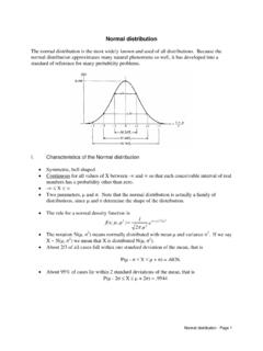
3 A . b-a 2 b-a 2. z f(z) dz The standard deviation of the uniform distribution is given by b 2. 2. b+a 1 (b - a). = E((X - ) ) = . 2 2. z - dz = (with some work!). a 2 b-a 12. (z- )2 f(z) dz II. normal distribution For a finite population the mean (m) and standard deviation (s) provide a measure of average value and degree of variation from the average value. If random samples of size n are drawn from the population, then it can be shown (the Central Limit Theorem) that the distribution of the sample means approximates that of a distribution with mean: = m s standard deviation: =.
4 N pdf: (x ) 2. 1 . f(x) = e 2 2. 2 . which is called the normal distribution . The pdf is characterized by its "bell- shaped" curve, typical of phenomena that distribute symmetrically around the mean value in decreasing numbers as one moves away from the mean. The "empirical rule" is that approximately 68% are in the interval [ - , + ]. approximately 95% are in the interval [ -2 , +2 ]. almost all are in the interval [ -3 , +3 ]. This says that if n is large enough, then a sample mean for the population is accurate with a high degree of confidence, since decreases with n.
5 What constitutes "large enough" is largely a function of the underlying population distribution . The theorem assumes that the samples of size n which are used to produce sample means are drawn in a random fashion. Measurements based on an underlying random phenomena tend to distribute normally. Hogg and Craig (Introduction to Mathematical Statistics) note that the kinds of phenomena that have been found to distribute normally include such disparate phenomena as 1) the diameter of the hole made by a drill press, 2) the score on a test, 3) the yield of grain on a plot of ground, 4) the length of a newborn child.
6 The assumption that grades on a test distribute normally is the basis for so-called "curving" of grades (note that this assumes some underlying random phenomena controlling the measure given by a test; , genetic selection). The practice could be to assign grades of A,B,C,D,F based on how many "standard deviations". separates a percentile score from the mean. Hence, if the mean score is , and the standard deviation is 8, then the curve of the class scores would be given by A: 94 and up ( ). B: 86-93 ( ). C: 70-85 (68%). D: 62-69 ( ). F: otherwise ( ).
7 Most people "pass", but A's are hard to get! This could be pretty distressing if the mean is 95 and the standard deviation is 2 ( , 90 is an F). A plot of the pdf for the normal distribution with = 30 and = 10 has the appearance: f(x). x .. Note that the distribution is completely determined by knowing the value of . and . The standard normal distribution is given by = 0 and = 1, in which case the pdf becomes x2. 1 2. f(x) = e 2 . nsample nsample z2. 1 2. x= 2 . e dz . nsample 0 x .5 1. It is sufficient to sample from the standard normal distribution , since the linear relationship rsample = + nsample substitute z= + t holds.
8 Dz = dt rsample (z- ) 2 + nsample ( + t - ) 2 + nsample t2. 1 - 1 1 2.. 2 . e 2. dz = . - 2 . e 2 2. dt = . - . 2 . e dt There is no "closed-form formula" for nsample, so approximation techniques have to be used to get its value. III. Exponential distribution The Exponential distribution arises in connection with Poisson processes. A. Poisson process is one exhibiting a random arrival pattern in the following sense: 1. For a small time interval t, the probability of an arrival during t is t, where = the mean arrival rate;. 2. The probability of more than one arrival during t is negligible.
9 3. Interarrival times are independent of each other. [this is a kind of "stochastic" process, one for which events occur in a random fashion]. Under these assumptions, it can be shown that the pdf for the distribution of interarrival times is given by f(x) = e - x which is the Exponential distribution . More to the point, if it can be shown that the number of arrivals during an interval is Poisson distributed ( , the arrival times are Poisson distributed), then the interarrival times are exponentially distributed. Note that the mean arrival rate is given by and the mean interarrival time is given by 1/.
10 The Poisson distribution is a discrete distribution closely related to the binomial distribution and so will be considered later. It can be shown for the Exponential distribution that the mean is equal to the standard deviation; , = = 1/ . Moreover, the Exponential distribution is the only continuous distribution that is "memoryless", in the sense that P(X > a+b | X > a) = P(X > b). f(x).. f(x) = e - x x rsample When = 1, the distribution is called the standard Exponential distribution . In this case, inverting the distribution is straight-forward; , nsample z nsample e dz = - e -z 0.