Introduction to LabVIEW for Control Design & …

1 Introduction to LabVIEW for Control Design & simulation Ricardo Dunia (NI), Eric Dean (NI), and Dr. Thomas Edgar (UT) Reference Text : Process Dynamics and Control 2nd edition, by Seborg, Edgar, Mellichamp, Wiley 2004 LabVIEW , which stands for Laboratory Virtual Instrumentation Engineering Workbench, is a graphical computing environment for instrumentation, system Design , and signal processing. The Control Design and simulation (CDSim ) module for LabVIEW can be used to simulate dynamic systems. To facilitate model definition, CDSim adds functions to the LabVIEW environment that resemble those found in SIMULINK.

2 There is also the ability to use m-file syntax directly in LabVIEW through the new MathScript node. The purpose of this tutorial is to introduce you to LabVIEW and give you experience simulating dynamic systems.. In the first section, you will build a model of the open-loop system for the second order plus time delay process 2()(10 1)(5 1)seGsss and determine the unit set-point and unit disturbance responses. In the second section, you will build a closed-loop model of the same process. After the closed-loop model is constructed, you should simulate the unit disturbance response and the unit set-point response for two different PID controller tuning methods, ITAE (set-point) and ITAE (disturbance), in Table (SEM).

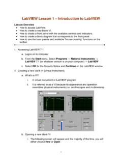
3 Log onto a PC computer. Click Start->National Instruments-> LabVIEW . Open LabVIEW . (Note : as of LabVIEW , the Control Design & simulation module is also supported for Mac ) Figure1. Initial LabVIEW Screen Start a new program (VI) Browse example VIs To start a new program ( called VI for Virtual Instrument ), click Blank VI Figure 2. LabVIEW new VI Click in the block diagram to view the area where graphical programs are written. Right-click inside the block diagram to view the palette of functions used in creating programs. Select the Control Design & simulation -> simulation palette to view the library of simulation functions.

4 Figure 3. simulation functions sub-pallette In Control Design & simulation pallette Block Diagram (programming window) Front Panel (user interface) In the next section, you will build a model of the open-loop system for the process mentioned earlier and determine the unit set-point and unit disturbance responses. The following steps will guide you through the discussed tasks. Construction of an Open-Loop Block Diagram (Chapters 4, 5, 6, and 7) 1. Open a new VI by selecting File->NewVI. The new window will be titled untitled. You will build your closed-loop model in the block diagram.

5 Save the empty model by choosing File->Save . Name the model, examplesim. From this point on, the model will be referred to as examplesim. 2. Click on the block diagram, then right-click to bring up the functions palette. From the simulation sub-pallette, click-and-drag a simulation loop on the block diagram. 3. Place the Transfer Function and Transport Delay blocks from the Continuous pallette, respectively, to Examplesim. Connect the output of the Transfer Function block to the input of the Transport Delay block. Click on the Transfer Function label and rename to Process TF.

6 This block represents the process. Note that in this problem, the process is G(s) = GvGpGm, not Gp. Click-and-drag to create simulation loop Open the dialog box of Process TF by double clicking on it. Specify Numerator as [2] and Denominator as [1 15 50]. This indicates the transfer function 2/(50s2 + 15s + 1). The Transfer Function block allows specification of vectors for the numerator and denominator from either a configuration dialog box, or a terminal from the block diagram. The vector elements are treated as the coefficients of ascending powers of s in the polynomials representing the numerator and denominator of the transfer function.

7 To see the denominator polynomial of s completely displayed in the block s icon, you may have to resize the block s icon. Double-click on the Transport Delay and set Time delay to 1. Note that the Transport Delay block can be used to represent other types, such as measurement delay. 4. Copy the Process TF and Transport Delay blocks and place the copies slightly above the originals. The copies will automatically change names to Process TF1 and Transfer Delay1 . To quickly copy the original blocks, select both of them, hold the CTRL key and drag using the left mouse button.

8 Rename the Process TF1 block Disturbance TF . In this example Gp and Gd are the same, so the Numerator and Denominator parameters in the dialog box of Disturbance TF are not changed (See Figure 4). 5. Place a copy of the Summation block, located in the Signal Arithmetic pallette, to the right of the Transport Delay block. Right-click on the summation block and select Visible Items->Label to see the label Summation . Connect the output from each Transport Delay block to the input of the Summation block. The number of inputs and their polarity can be modified from the dialog box.

9 Later in the tutorial you will be required to do this. 6. Place a SimTime Waveform graph, from the Graph Utilities palette, to the right of the Summation block. Connect the output of the Summation block to the input of the SimTime Waveform block. 7. Place a Step Signal block, from the Signal Generation palette, to the left of Disturbance TF and connect it to the input of Disturbance TF. The Step Signal block generates a step function. The initial value, final value and step time (time at which the step occurs) of the function can be specified. For now, double-click to open its dialog box and set the initial value, and final value, and step time to zero, , disabling the block.

10 Rename the block D . 8. Place a copy of D to the far left of Process TF and rename the new block U . Connect U to the input of Process TF. Double-click on U and set Step time to 0, Initial value to 0 and Final value 1. U will generate a unit step function in the manipulated variable at time zero. The model developed to this point is a model of the open-loop system. It should look similar to the model below. 9. Now we are ready to simulate the open-loop response of the system. To select the integration technique and parameters to be used during simulations, double-click on the left terminal of the simulation loop.