Transcription of STATE-FEEDBACK CONTROL
1 ECE4520/5520: Multivariable CONTROL Systems 1 STATE-FEEDBACK : STATE-FEEDBACK CONTROL We are given a particular system having : We know that open-loop system poles are given by eigenvaluesofA. Want to use change the dynamics. Will assume the form oflinearstatefeedback with gain ! ; K2R1"n: We assume known exactly: then, we ; B; C; DxK ! ! : For now we talk about regulation ( ) notes prepared by Dr. Gregory L. Plett. Copyrightc#2015, 2011, 2009, 2007, 2005, 2003, 2001, 2000, Gregory L. PlettECE4520/5520, STATE-FEEDBACK CONTROL6 2 For now we consider SISO systems, and generalize :DesignKso thatACLDA!BKhas some nice example, PerhapsAis unstable. DesignACLto be stable. Or, might want to put two poles at!2 j.(Poleplacement.) There arenparameters in the gain vectorKandneigenvalues , what can we achieve?
2 EXAMPLE:Consider the (unstable) "1112# "10# ! !1/.s!2/!1Ds2!3sC1: ! ! !BKD"1112#!"10#hk1k2iD"1!k11!k212#: So, ! !3 !2k1Ck2/. By choosingk1andk2, the complexplane (in complex-conjugate pairs, that is!) For example, how can we place poles at!5;!6?Lecture notes prepared by Dr. Gregory L. Plett. Copyrightc#2015, 2011, 2009, 2007, 2005, 2003, 2001, 2000, Gregory L. PlettECE4520/5520, STATE-FEEDBACK CONTROL6 3 Compare desired closed-loop characteristic ! !3 !2k1Ck2/: So,k1!3D11;or;k1D141!2k1Ck2D30;or;k2D57: KD 14 57 . So, with thenparameters inK, $Most physical systems, qualified yes.$Mathematically, EMPHATIC NO! Boils down to whether or not the system is, ifevery internal system mode can be excited by inputs, either directly :Consider the "1102# "10# ! :ACLDA!BKD"1!k11!k202# ! !1Ck1/.s!2/: feedback of the state cannot move the pole stabilized via state feedback .
3 (Note that the system is already inKalman form, and the uncontrollable mode has eigenvalue 2).Lecture notes prepared by Dr. Gregory L. Plett. Copyrightc#2015, 2011, 2009, 2007, 2005, 2003, 2001, 2000, Gregory L. PlettECE4520/5520, STATE-FEEDBACK CONTROL6 : Bass Gura pole placementFACT:IffA; Bgis controllable, then we can arbitrarily assign theeigenvalues ofACLusing state feedback . More precisely, given anypolynomialsnC 1sn!1C%%%C nthere exists a (unique for SISO)K2Rm"n(mDnumber of system inputsD1for SISO) such !ACBK/DsnC 1sn!1C%%%C n:COROLLARY:IffA; Bgis controllable, we can find a state feedback forwhich the closed-loop realization is OF FACT:We prove this by solving for the state feedback vectorKto put the poles where we desire. First, supposefA; Bgis controllable. To make a hard problem easier, we then transformfA; B; C; Dgintocontroller canonical form.
4 (Then solve problem in this form, thenconvert back to original form). That is, findTsuch thatT!1 ATDAcD266664!a1!a2%%%!an10::::::0%%%1037 7775andT!1 BDBcD26666410 !A/DsnCa1sn!1C%%%Can.$We defer calculation ofTfor now. Let s apply state-feedbackKcto the controller notes prepared by Dr. Gregory L. Plett. Copyrightc#2015, 2011, 2009, 2007, 2005, 2003, 2001, 2000, Gregory L. PlettECE4520/5520, STATE-FEEDBACK CONTROL6 5 Note,KcDhk1%%%kni,soBcKcD266664k1k2%%%kn 00::::::00377775: Useful because characteristic equation !BcKcD266664!.a1Ck1/!.a2Ck2/%%%!.anCkn/1 0::::::0%%%10377775;still in controller form! !a1!a2!a3!k1!k2!k3 Thus, after state feedback withKcthe characteristic equation ! !1C%%% :Lecture notes prepared by Dr. Gregory L. Plett. Copyrightc#2015, 2011, 2009, 2007, 2005, 2003, 2001, 2000, Gregory L.
5 PlettECE4520/5520, STATE-FEEDBACK CONTROL6 6 The desired characteristic equation is" 1sn!1C%%%C n: Equating coefficients of powers-of-s,wesetk1D 1!a1;:::;knD n!anand get the desired characteristicpolynomial. Now that we have the solution in the controller canonical form, wetransform back to the original realization" ! ! !1 !TAcT!1 CTBcKcT!1 !ACBKcT!1/:". !ACBK/soKDKcT!1:So, if we use state feedbackKDKcT!1Dh. 1!a1/%%%. n!an/iT!1we will have the desired characteristic polynomial. One remaining question: What isT?WeknowTDCC!1candCcD2666641!a1a21!a2% %%01!a10:::1:::0%%%1377775 Lecture notes prepared by Dr. Gregory L. Plett. Copyrightc#2015, 2011, 2009, 2007, 2005, 2003, 2001, 2000, Gregory L. PlettECE4520/5520, STATE-FEEDBACK CONTROL6 7C!1cD2666641a1%%%an!101:::::::::a101377 775 ..upper ToeplitzT!
6 1D2666641a1%%%an!101:::::::::a101377775! 1C!1 So,KDh. 1!a1/%%%. n!an/i2666641a1%%%an!101 an!2:::::::::01377775!1C!1: This is called theBass Gura notes prepared by Dr. Gregory L. Plett. Copyrightc#2015, 2011, 2009, 2007, 2005, 2003, 2001, 2000, Gregory L. PlettECE4520/5520, STATE-FEEDBACK CONTROL6 : Ackermann s formula We need to knowaito use the Bass Gura formula. Ackermann smethod may require less work. Consider (a system already in controller canonical form, fornow),".s/DsnCa1sn!1C%%%Cans0".Ac/DAnc Ca1An!1cC%%%CanID0by Cayley Hamilton. Also," 1sn!1C%%%C ns0" 1An!1cC%%%C nI 0" !0D" !".Ac/D. 1!a1/An!1cC%%%C. n!an/I: Asneakyfactforthecontrollerformis,h0%%%1 iAkcDh0%%%1 ..n!k%%%0iso thath0%%%1i" 1!a1/. 2!a2/%%%. n!an/iDKcKcDh0%%%1i" : To convert to the original form,KDKcT!1Dh0%%%1i" !1AT /T!
7 1Dh0%%%1iT!1" notes prepared by Dr. Gregory L. Plett. Copyrightc#2015, 2011, 2009, 2007, 2005, 2003, 2001, 2000, Gregory L. PlettECE4520/5520, STATE-FEEDBACK CONTROL6 9Dh0%%%1iCcC!1" !1" : Revisit previous example." "1101#KDh01i"1!101#("1112#"1112#C11"1112 #C30"1001#)Dh01i("2335#C"41 1111 52#)Dh01i"43 1414 57#Dh14 57i: same as before: K=acker(A,B,poles); Very easy in Matlab, but numericalissues. K=place(A,B,poles); Use this instead, unless you haverepeated roots. To compute" state feedback in Simulink The following block diagram may be used to simulate astate- feedback CONTROL system in notes prepared by Dr. Gregory L. Plett. Copyrightc#2015, 2011, 2009, 2007, 2005, 2003, 2001, 2000, Gregory L. PlettECE4520/5520, STATE-FEEDBACK CONTROL6 10 Note: All (square) gain blocks are MATRIX GAIN blocks from the Math commentsFACT:The eigenvalues associated with uncontrollable modes are fixed(don t change) under state feedback , but those associated withcontrollable modes can be arbitrarily :State feedback does not change zeros of a :Drastic changes in characteristic polynomial requires large gainsK(high CONTROL effort).
8 FACT:State feedback can result in unobservable modes (pole-zerocancellations).Lecture notes prepared by Dr. Gregory L. Plett. Copyrightc#2015, 2011, 2009, 2007, 2005, 2003, 2001, 2000, Gregory L. PlettECE4520/5520, STATE-FEEDBACK CONTROL6 : Reference input So far, we have looked at how to pickKto get homogeneousdynamics that we !fast=slow=real poles:::How does this improve our ability to track a reference? Started ! good tracking. Frequency domain, low frequencies. Problem is ! simple, but it :AD"1112#;BD"10#;KDh14 57i: !ACBK/! "sC13 56!1s!2#!1"10#Dh10i"s!2!561sC13#s2C11s!2 6C56"10#Ds!2s2C11sC30: Final value theorem for step input, !!230 1!Lecture notes prepared by Dr. Gregory L. Plett. Copyrightc#2015, 2011, 2009, 2007, 2005, 2003, 2001, 2000, Gregory L. PlettECE4520/5520, STATE-FEEDBACK CONTROL6 12012345678910 ResponseAmplitudeTime (sec.)
9 OBSERVATION:Aconstantoutputyssrequires constant statexssandconstant problem !uss/D! !xss/: ussandxssrelated ..1"1rssxssDNx ..n"1rss: How to findNuandNx? : At steady state, ANxCBNu CNxCDNu rss: Two equations and two notes prepared by Dr. Gregory L. Plett. Copyrightc#2015, 2011, 2009, 2007, 2005, 2003, 2001, 2000, Gregory L. PlettECE4520/5520, STATE-FEEDBACK CONTROL6 13"ABCD#"NxNu#D"0I#: In steady-state we !uss/D! !xss/which is achieved by the CONTROL ! ! ! ! : NNcomputed without In our example we can find that"NxNu#D2641!1=2!1=2375: NuCKNxD!15: New ! ! : Therefore,! "newD! "old"NND!15sC30s2C11sC30which has zero steady-state error to a notes prepared by Dr. Gregory L. Plett. Copyrightc#2015, 2011, 2009, 2007, 2005, 2003, 2001, 2000, Gregory L. PlettECE4520/5520, STATE-FEEDBACK CONTROL6 ; B; C; DA; B; C; DxxKKNNNxNu Simulate (either method)012345678910 ResponseAmplitudeTime (sec.)
10 Lecture notes prepared by Dr. Gregory L. Plett. Copyrightc#2015, 2011, 2009, 2007, 2005, 2003, 2001, 2000, Gregory L. PlettECE4520/5520, STATE-FEEDBACK CONTROL6 : Pole placement Classical question: Where do we place the closed-loop poles?THOUGHT I:Dominant second-order behavior, just as before. Assume dominant behavior given by roots ofs2C2$!nsC!2n sD!n!n j!np1!$2o Put other poles so that the time response is much faster than thisdominant behavior. Place them so that they are sufficiently damped. $Real part<!4$!n.$Keep frequency same as open loop. Be very careful about moving poles too far. Takes a lot of II:Can also choose closed-loop poles to mimic a system thathas performance that you like. Set closed-loop poles equal tothisprototype system. Scaled to give settling time of 1 sec. or bandwidth of!