Transcription of Chapter 5 Testing Converters F - Analog Devices
1 Testing DATA Converters Analog -DIGITAL CONVERSION 1. Data Converter History 2. Fundamentals of Sampled Data Systems 3. Data Converter Architectures 4. Data Converter Process Technology 5. Testing Data Converters Testing DACs Testing ADCs 6. Interfacing to Data Converters 7. Data Converter Support Circuits 8. Data Converter Applications 9. Hardware Design Techniques I. Index Analog -DIGITAL CONVERSION Testing DATA Converters Testing DACS Chapter 5 Testing DATA Converters SECTION : Testing DACs Walt Kester, Dan Sheingold Static DAC Testing The resolution of a DAC refers to the number of unique output voltage levels that the DAC is capable of producing. For example, a DAC with a resolution of 12 bits will be capable of producing 212 or 4,096 different voltage levels at its output .
2 Similarly, a DAC with a resolution of 16 bits can produce 216 or 65,536 levels at its output . Inherent in the specification of resolution, especially for control applications, is the requirement for monotonicity. The output of a monotonic DAC always stays the same or increases for an increasing digital code. The quantitative measure of monotonicity is the specification of differential nonlinearity (step size). The static absolute accuracy of a DAC can be described in terms of three fundamental kinds of errors: offset errors, gain errors, and integral nonlinearity. Linearity errors are the most important of the three kinds, because in many applications the user can adjust out the offset and gain errors, or compensate for them without difficulty by building end-point auto-calibration into the system design, whereas linearity errors cannot be conveniently or inexpensively nulled out.
3 But before we can understand the nature of linearity errors and how to test for them, the end-point errors must first be established. There are many methods to measure the static errors of a DAC the proper choice depends upon the specific objectives of the Testing . For instance, an IC manufacturer generally performs production Testing on DACs using specialized automatic test equipment. On the other hand, a customer evaluating various DACs for use in a system does not generally have access to sophisticated automatic test equipment and must therefore devise a suitable bench test setup. A basic DAC static test setup is shown in Figure This flexible test setup allows the application of various digital codes to the DAC input and uses an accurate digital voltmeter for measuring the DAC output .
4 Computer control can be used to automate the process, but it should be noted that in many cases DAC static Testing can be performed by simply using mechanical switches to apply various codes to the DAC and reading the output with the voltmeter. Today there are a large number of applications where the static performance of a DAC is rarely of direct concern to the customer even in the evaluation phase and ac performance is much more important. DACs used in audio and communications quite often do not even have traditional static specifications listed on the data sheet, and various noise and distortion specifications are of much more interest. However, the Analog -DIGITAL CONVERSION traditional static specifications such as differential nonlinearity (DNL) and integral nonlinearity (INL) are most certainly reflected in the ac performance.
5 For instance, low distortion, a key audio and communication requirement, is directly related to low INL. Large INL and DNL errors will increase both the noise and distortion level of a DAC and render it unsuitable for these demanding applications. In fact, one often finds that the static performance of these ac-specified DACs is quite good, even though it is not directly specified. Figure : Basic Test Setup for Measuring DAC Static Transfer Characteristics The following sections on static DAC Testing are therefore more oriented to DACs which are used in traditional industrial control, measurement, or instrumentation applications where monotonicity, DNL, INL, gain, and offset are important. End-Point Errors The most commonly specified end-point errors associated with DACs are offset error, gain error, and bipolar zero error.
6 Note that bipolar zero error is only associated with bipolar output DACs, whereas offset and gain error is common to both unipolar and bipolar DACs. Figure shows the effects of offset and gain error in a unipolar DAC. Note that in Figure , all output points are offset from the ideal (shown as a dotted line) by the same amount. Any such error either positive or negative that affects all output points by the same amount is an offset error. The offset error can be measured by applying the all "0"s code to the DAC and measuring the output deviation from 0 volts. Figure shows the effect of gain error only. The ideal transfer function has a slope defined by drawing a straight line through the two end points. The slope represents the gain of the transfer function. In non-ideal DACs, this slope can differ from the ideal, resulting in a gain error which is usually expressed as a percent because it affects each LOGIC ANDREGISTERSPRECISIONVOLTMETERCOMPUTERTI MINGPARALLELOR SERIALDATAINTERFACEN-BITDACBUS:IEEE-488, USB, RS-232, DATA Converters Testing DACS code by the same percentage.
7 If there is no offset error, gain error is easily determined by applying the all "1"s code to the DAC and measuring its output , designated as V111 (assuming a 3-bit DAC). An ideal DAC will measure exactly VFS 1 LSB, so the gain error is computed using the equation: =1 LSB1VV100(%)ErrorGainFS111. Eq. Figure : Measuring Offset and Gain Error in a Unipolar DAC Figure shows the case where there is both offset and gain error. The first step is to measure the offset error, VOS, by applying the all "0"s code and measuring the output . Next, apply the all "1"s code and measure the output V111. The gain error is then calculated using the equation: =1 LSB1 VVV100(%)ErrorGainFSOS111. Eq.
8 Figure shows how gain and offset errors affect the ideal transfer function of a bipolar output DAC. The offset error in Figure , VOS, is measured by applying the all "0"s code to the DAC input and measuring the output . Ideally, the DAC should have an output of FS with all "0"s at its input . The difference between the actual output and FS is the offset, VOS. In a bipolar DAC it is also common to specify and measure the bipolar zero error (or zero error) because of its importance in many applications. It is measured by applying the mid-scale code 100 to the DAC and measuring its output . If there is no gain error, the bipolar zero error is the same as the offset error as shown in Figure DIGITAL CODE INPUTDIGITAL CODE INPUTDIGITAL CODE INPUT000111000111000111 VOSVOSV111V111V111 VFS 1 LSBVFS 1 LSBVFS 1 LSBOFFSET ERROR = V000= VOSGAIN ERROR = 0 OFFSET ERROR = 0 GAIN ERROR (%) =V111 VFS 1 LSB 1100 OFFSET ERROR = V000 = VOSGAIN ERROR (%) =V111 VOSVFS 1 LSB 1100(A) OFFSET ERROR(B) GAIN ERROR(C) OFFSET ANDGAIN ERRORIDEALIDEALIDEAL00 0 Analog -DIGITAL CONVERSION Figure : Measuring Offset, Bipolar Zero, and Gain Error in a Bipolar DAC Figure shows the case where there is gain error, but no offset error.
9 Notice that the bipolar zero error is affected by the gain error. The DAC output V111 is measured by applying the all "1"s code, and the gain error is calculated from the equation: +=1 LSB1V2VV100(%)ErrorGainFSFS111. Eq. The bipolar zero error is determined by applying 100 to the DAC and measuring its output . Figure shows the case where the bipolar DAC has both gain and offset error. The offset error is determined as above by applying the all "0"s code, measuring the DAC output , and subtracting it from the ideal value, VFS. The all "1"s code is applied to the DAC and the output V111 is measured. The gain error is calculated using the equation: +=1 LSB1V2 VVV100(%)ErrorGainFSOSFS111. Eq.
10 The bipolar zero error is determined by applying 100 to the DAC and measuring its output . Bipolar zero error in DACs using offset-type coding is a derived, rather than a fundamental quantity, because it is actually the sum of the bipolar offset error, the bipolar DIGITAL CODE INPUT111 VOSV111 VFS 1 LSBOFFSET ERROR = VOS= V000+VFSGAIN ERROR = 0 OFFSET ERROR = 0 GAIN ERROR (%) =V111+ VFS2 VFS 1 LSB 1100 GAIN ERROR (%) =V111 + VFS VOS2 VFS 1 LSB 1100 VFS100 DIGITAL CODE INPUT111 VOS= 0V111 VFS 1 LSB VFS100 DIGITAL CODE INPUT111 VOSV111 VFS 1 LSB VFS100(A) OFFSET ERROR(B) GAIN ERROR(C) OFFSET ANDGAIN ERRORBIPOLARZERO ERROR= VOSBIPOLARZERO ERRORBIPOLARZERO ERRORIDEALIDEALIDEAL000000000000 OFFSET ERROR = VOS= V000+VFSBIPOLAR ZERO ERROR = V100 =VOSBIPOLAR ZERO ERROR = V100 BIPOLAR ZERO ERROR = V100 Testing DATA Converters Testing DACS gain error, and the MSB linearity error.