Transcription of ChapterII RF-CIRCUITS
1 Class Notes, 31415 RF-Communication Circuits Chapter IIRF-CIRCUITSJens Vidkj rNB230 iiContentsII RF-CIRCUITS , Concepts and 1II-1 parallel Resonance 2 Frequency 3 Poles and 6 Transient 8II-2 Series Resonance circuit 11II-3 Narrowband 14II-4 Series-to- parallel 19 Example II-4-1 ( impedance matching ).. 20 Conversions in Narrowband 23 Conversions in Broadband 26 Example II-4-2 ( spiral inductor ).. 26II-5 Tuned 30 Synchronously Tuned 32 Example II-5-1 ( synchronous tuning ).. 33 Butterworth Stagger Tuned 36 Example II-5-2 ( Butterworth amplifier ).. 41II-6 Transformers and Transformerlike 45 Review of Mutual 45 Equivalent Circuits for Two Coupled 53 Example II-6-1 ( practical RF transformers ).
2 55 Tuned 57 Example II-6-2 ( transformer-coupled tuned amplifier ).. 61 Example II-6-3 ( autotransformers in a tuned amplifier ) .. 62 Transformerlike 63 Example II-6-4 ( uncoupled reactance transformers intuned amplifiers ).. 64 Three-Winding 67 Transformer 72 Example II-6-5 ( diode-ring mixer preliminaries ).. 78II-7 Double-Tuned Circuits and 80 Coupling between Identical Resonance 81 Example II-7-1 ( Foster-Seely FM detector ).. 85 Example II-7-2 ( quadrature FM detector ).. 88 Double-Tuned Amplifier 94 Asymptotic 98II-8 Impedance riiiLumped Element Impedance Matching using Smith II-8-1 ( double and standard Smith charts )..104 Example II-8-2 ( bandwidth estimations )..108 APPENDIX II-A, Power Calculation and Power II-B Signal Flow Signal Flow s Direct and Further riv1II RF-CIRCUITS , Concepts and MethodsIn RF-communication system, control of frequency bands and impedance matchingconditions between functional blocks or amplifier stages are problems that constantly face acircuit designer.
3 The tasks are so frequent that many analytical techniques and approximationmethods especially suited for high-frequency circuits have evolved and strongly influenced thejargon of RF engineering. Below we shall introduce the most important basic concepts andmethods that are required to- understand data sheets and literature,- make simpler design decisions or calculations, and- prepare and interpret simulation selection of topics and examples have furthermore been conducted to suit the needs inthe following chapters, which are still in contents, the chapter starts summarizing basic properties of resonancecircuits. Although significant by themselves, the importance of acquiring familiarity with idealresonance circuits is the fact, that any narrowbanded resonance circuit may be approximatedby the ideal ones around resonance frequencies.
4 This property reduces significantly the effortsthat are required to understand and explore operations of tuned bandpass circuits, which arefrequently used in RF-communication systems. Foundations of the simplifications are dealtwith in sections concerning narrowband approximations and series-to- parallel tuned amplifiers are introduced in ideal form concentrating on simple frequency charac-teristics. Coupling techniques using transformers and coupled resonance circuits are still highlyuseful methods in RF-designs, so they are considered in some details here. Finally, the verygeneral method of constructing lumped element matching networks using a Smith chart matching is fundamental for designing and understanding many RF this concept is mandatory in basic circuit theory curriculums, it is repeated forconvenience in an appendix.
5 Also the method of illustrating and solving network equationsby the signal flow graph method is summarized in an r2II-1 parallel Resonance parallel resonance circuit (1)A basic parallel resonance circuit is shown in Besides component values thecombinations, which are summarized by Eq.(1), are frequently used. The resonance frequencyis the frequency where the capacitive and the inductive susceptances are equal in magnitudeas indicated in When an external steady state sinusoidal voltage-source of frequency 0is applied to the resonance circuit , the two opposite currents through the capacitor and theinductor balance each other, and only the resistor current flows through the terminal. Thissituation is sketched in , which also shows how the quality factor Q indicates themagnitude ratio of the internal reactive currents over the resistive terminal current at resonance.
6 (a) Susceptance composition as function of frequency. (b)Current and voltage phasors at the resonance frequency view upon resonance and the quality factor concerns the energy in the circuitunder steady state conditions. At instants where the two phasors iCand iLare perpendicularto the real axis, no currents flow into the capacitor or inductor, but the capacitor holdmaximum energy(2) r3II-1 parallel Resonance CircuitsThe first equation is the usual electrostatic energy expression. The second takes into accountthat rms values - indicated by small letters - are conventionally used when dealing with steadystate linear circuits. A quarter of a period later the current phasors project in full onto the realaxis while the voltage is zero.
7 The capacitor holds no energy, but the inductor energy peakswith the same maximum that formerly was held in the capacitor,Thus, a constant amount of energy laps between the capacitor and the inductor at resonance,(3)and the quality factor may be expressedwhere the loss is calculated as the resistor power times the resonance period T0=2 / 0. This(4)interpretation of resonance is often useful in the construction of lumped circuit equivalents forthe variety of electromagnetic and mechanical resonators that are used in ResponseExpressed through circuit element values, the impedance function for the parallelcircuit in isIntroducing 0and Q from Eq.(1), the impedance expressed as a function of frequency s=j (5)becomesThe frequency dependency of the impedance is kept in the quantity ( ), which is zero at the(6)resonance frequency 0.
8 Here the denominator of Eq.(6) gets its smallest size and theimpedance has maximum Rp, the parallel resistance. The magnitude and phase of Zp(j ) areThe two functions are shown in (a) while (b) shows the corresponding admittance(7)characteristics, r4RF-Circuits, Concepts and MethodsUpper and lower bounds of the 3dB bandwidth intervals W3dB,which are (a) and admittance (b) magnitudes and phases of the parallel resonancecircuit in The curves are symmetric around odue to the logarithmic fre-quency scales.(8)in , correspond to a denominator size equal to 2 in Eq.(7). The bounds are foundsetting the imaginary part of the denominator equal in magnitude to the real part, negative and positive frequencies are contained in the conditions.
9 We call the largest(9)valued solutions, where the two terms in bhave equal signs, the upper bounds bu. Thelower bounds blare obtained with terms of opposite signs. summarizes how thedifferent solutions are formed. By definition, the 3dB bandwidth is taken to be the distancebetween positive or zero-valued 3dB frequency bounds, and we get the result that wasincorporated in ,It follows from the solutions in Eq.(9) that the resonance frequency 0is not centered between(10)the 3dB bounds but is the geometrical mean of the bounds, r5II-1 parallel Resonance Upper and lower 3dB bound positions from Eq.(9) . Note, in linear frequency scalethe 3dB bands are not symmetric around the resonances at 0unless Q .(11)so in logarithmic frequency scale the upper and lower 3dB frequency bounds are symmetric(12)with respect to log 0.
10 However, any other pair of frequencies, u, lthat has the resonancefrequency as geometrical mean maps symmetrically around log 0. Since both frequenciesprovide the same absolute | |, impedance or admittance magnitude characteristics of the types in have even(13)symmetry with respect to the resonance frequency in a logarithmic frequency scale. Corre-spondingly, the phase characteristics show odd symmetry because tan-1(-Q )=-tan-1(Q ). Atthe 3dB boundaries where |Q |=1, the phase angles of impedance Zpbecome . plots of the impedance function with various Q-factors. The normalization in magnitudecorresponds to keeping the inductor and capacitor fixed while letting the parallel resistancefollows Q according to Eq.(1). The asymptotic behavior of the impedance approximating theinductor reactance below and the capacitor reactance above resonance respectively are readilyobserved.